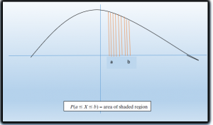
11 Facts On Mathematical Expectation & Random Variable

2 1

Mathematical Expectation and random variable    

     The mathematical expectation plays very important role in the probability theory, the basic definition and basic properties of mathematical expectation already we discussed in previous some articles now after discussing the various distributions and types of distributions, in the following article we will get familiar with some more advanced properties of mathematical expectation.

Expectation of sum of random variables | Expectation of function of random variables | Expectation of Joint probability distribution

     We know the mathematical expectation of random variable of discrete nature is

2 1
2.0 Copy

and for the continuous one is

3.0 Copy

now for the random variable X and Y if discrete then with the joint probability mass function p(x,y)

expectation of function of random variable X and Y will be

4.0

and if continuous then with the joint probability density function f(x, y) the expectation of function of random variable X and Y will be

5.0

if g is addition of these two random variables in continuous form the

6.0
7.0
8.0
9.0

and if for the random variables X and Y we have

X>Y

then the expectation also

10.0 1

Example

A Covid-19 hospital is uniformly distributed on the road of the length L at a point X, a vehicle carrying oxygen for the patients is at a location Y which is also uniformly distributed on the road, Find the expected distance between Covid-19 hospital and oxygen carrying vehicle if they are independent.

Solution:

To find the expected distance between X and Y we have to calculate E { | X-Y | }

Now the joint density function of X and Y will be

11.0 1

since

12.0 1

by following this we have

13.0 1

now the value of integral will be

14.0
15.0
16.0

Thus the expected distance between these two points will be

17.0

Expectation of Sample mean

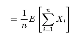
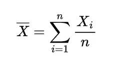
  As the sample mean of the sequence of random variables X1, X2, ………, Xn with distribution function F and expected value of each as μ is

18.0

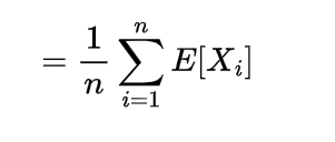
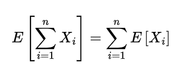
so the expectation of this sample mean will be
19.0
20.0
71.0
22.0

which shows the expected value of sample mean is also μ.

Boole’s Inequality

                Boole’s inequality can be obtained with the help of properties of expectations, suppose the random variable X defined as
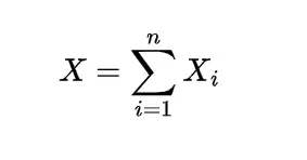
23.0 1

where

24.0

here Ai ‘s are the random events, this means random variable X represents the occurrence of the number of events Ai and another random variable Y as
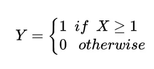
25.0

clearly

X>=Y

E[X] >= E[Y]

and so is

now if we take the value of random variable X and Y these expectation will be

28.0

and

29.0

substituting these expectation in the above inequality we will get Boole’s inequality as

30.0

Expectation of Binomial random variable | Mean of Binomial random variable

  We know that the binomial random variable is the random variable which shows number of successes in n independent trials with probability of success as p and failure as q=1-p, so if

X=X1 + X2+ …….+ Xn

Where

31.0

here these Xi ‘s are the Bernoulli and the expectation will be

32.0

so the expectation of X will be

33.0

Expectation of Negative binomial random variable | Mean of Negative binomial random variable

  Let a random variable X which represents the number of trials needed to collect r successes, then such a random variable is known as negative binomial random variable and it can be expressed as

34.0

here each Xi denote the number of trials required after the (i-1)st success  to obtain the total of i successes.

Since each of these Xi represent the geometric random variable and we know the expectation for the geometric random variable is

35.0

so

36.0

which is the expectation of negative binomial random variable.

Expectation of hypergeometric random variable | Mean of hypergeometric random variable

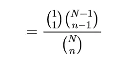
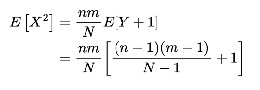
The expectation or mean of the hypergeometric random variable we will obtain with the help of a simple real life example, if n number of books are randomly selected from a shelf containing N books of which m are of mathematics, then to find the expected number of mathematics books let X denote the number of mathematics books selected then we can write X as

37.0

where

38.0

so

39.0
40.0

=n/N

which gives

41.0

which is the mean of such a hypergeometric random variable.

Expected number of matches

   This is very popular problem related to expectation, suppose that in a room there are N number of people who throw their hats in the middle of the room  and all the hats are mixed  after that each person randomly choose one hat then the expected number of people who select their own hat we can obtain by letting X to be the number of matches so

42.0

Where

43.0

since each person has equal opportunity to select any of the hat from N hats then

44.0

so

45.0

which means exactly one person on average choose his own hat.

The probability of a union of events

     Let us obtain the probability of the union of the events with the help of expectation so for the events Ai

46.0

with this we take

47.0

so the expectation of this will be

48.0

and expanding using expectation property as

49.0

since we have

Mathematical Expectation
Mathematical Expectation: The probability of a union of events

and

51.0

so

52.0

this implies the probability of union as

52.0 1

Bounds from Expectation using Probabilistic method

    Suppose S be a finite set and f is the function on the elements of S and

53.0

here we can obtain the lower bound for this m by expectation of f(s) where “s” is any random element of S whose expectation we can calculate so

54.0
55.0 1

here we get expectation as the lower bound for the maximum value

Maximum-Minimum identity

 Maximum Minimum identity is the maximum of the set of numbers to the minimums of the subsets of these numbers that is for any numbers xi

56.0 1

To show this let us restrict the xi within the interval [0,1], suppose a uniform random variable U on the interval (0,1) and the events Ai as the uniform variable U is less than xi that is

57.0

since at least one of the above event occur as U is less than one the value of xi

58.0

and

59.0

Clearly we know

60.0

and all the events will occur if U is less than all the variables and

62.0 1

the probability gives

62.0

we have the result of probability of union as

63.0

following this inclusion exclusion formula for the probability

64.0

consider

65.0

this gives

66.0

since

67.0

which means

68.0
  • hence we can write it as
69.0

taking expectation we can find expected values of maximum and partial minimums as

70.0

Conclusion:

The Expectation in terms of various distribution and correlation of expectation with some of the probability theory concepts were the focus of this article which shows the use of expectation as a tool to get expected values of different kind of random variables, if you require further reading go through below books.

For more articles on Mathematics, please see our Mathematics page.

https://en.wikipedia.org/wiki/Expectation

A first course in probability by Sheldon Ross

Schaum’s Outlines of Probability and Statistics

An introduction to probability and statistics by ROHATGI and SALEH

Conditional Distribution: 7 Interesting Facts To Know

9.PNG

Conditional distribution

   It is very interesting to discuss the conditional case of distribution when two random variables follows the distribution satisfying one given another, we first briefly see the conditional distribution in both the case of random variables, discrete and continuous then after studying some prerequisites we focus on the conditional expectations.

Discrete conditional distribution

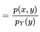
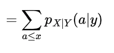
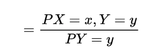
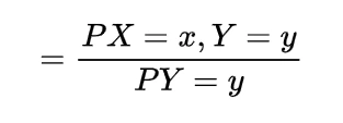
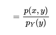
     With the help of joint probability mass function in joint distribution we define conditional distribution for the discrete random variables X and Y using conditional probability for X given Y as the distribution with the probability mass function

1
2.PNG
3.PNG

provided the denominator probability is greater than zero, in similar we can write this as

4.PNG
5.PNG

in the joint probability if the X and Y are independent random variables then this will turn into

6.PNG
7.PNG
8.PNG

so the discrete conditional distribution or conditional distribution for the discrete random variables X given Y is the random variable with the above probability mass function in similar way for Y given X we can define.

Example on discrete conditional distribution

  1. Find the probability mass function of random variable X given Y=1, if the joint probability mass function for the random variables X and Y has some values as

p(0,0)=0.4 , p(0,1)=0.2, p(1,0)= 0.1, p(1,1)=0.3

Now first of all for the value Y=1 we have

9.PNG

so using the definition of probability mass function

10.PNG
11.PNG
12.PNG

we have

13.PNG

and

14.PNG
  • obtain the conditional distribution of X given X+Y=n, where X and Y are Poisson distributions with the parameters λ1 and λ2 and X and Y are independent random variables

Since the random variables X and Y are independent, so the conditional distribution will have probability mass function as

15.PNG
16.PNG
17.PNG

since the sum of Poisson random variable is again poisson so

18.PNG
19.PNG
20.PNG

thus the conditional distribution with above probability mass function will be conditional distribution for such Poisson distributions. The above case can be generalize for more than two random variables.

Continuous conditional distribution

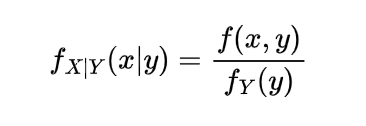
   The Continuous conditional distribution of the random variable X given y already defined is the continuous distribution with the probability density function

21.PNG

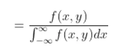
denominator density is greater than zero, which  for the continuous density function is

22.PNG
23.PNG

thus the probability for such conditional density function is

24.PNG

In similar way as in discrete if X and Y are independent  in continuous then also

25.PNG

and hence

px 26
px 28 Copy 1

so we can write it as

px 29 Copy 1

Example on Continuous conditional distribution

  1. Calculate conditional density function of random variable X given Y if the joint probability density function with the open interval (0,1) is given by
px 30 Copy 1

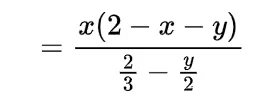
If for the random variable X given Y within (0,1) then by using the above density function we have

px 31
px 32
px 33
px 34
px 35
  • Calculate the conditional probability
px 36

if the joint probability density function is given by

px 37

To find the conditional probability first we require the conditional density function so by the definition it would be

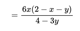
px 38
px 39
px 40

now using this density function in the probability the conditional probability is

100
101
px 41

Conditional distribution of bivariate normal distribution

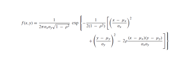
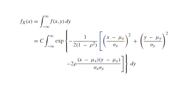
  We know that the Bivariate normal distribution of the normal random variables X and Y with the respective means and variances as the parameters has the joint probability density function

Conditional distribution
Conditional distribution of bivariate normal distribution

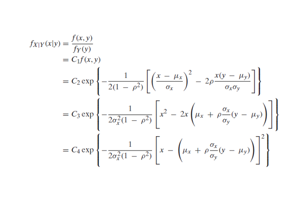
so to find the conditional distribution for such a bivariate normal distribution for X given Y is defined by following the conditional density function of the continuous random variable and the above joint density function we have

Conditional distribution
Conditional distribution of bivariate normal distribution

By observing this we can say that this is normally distributed with the mean

px 42

and variance

px 43

in the similar way the conditional density function for Y given X already defined will be just interchanging the positions of the parameters of X with Y,

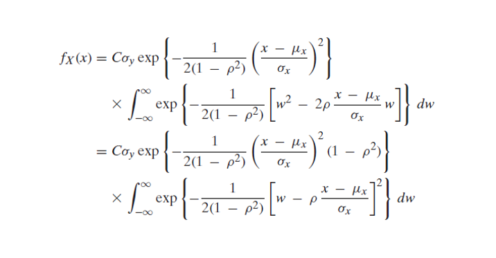
The marginal density function for X we can obtain from the above conditional density function by using the value of the constant

Conditional distribution
Conditional distribution of bivariate normal distribution

let us substitute in the integral

px 44

the density function will be now

Image3 1

since the total value of

Image4

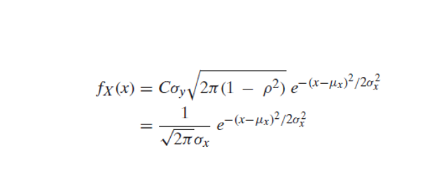
by the definition of the probability so the density function will be now

Image5

which is nothing but the density function of random variable X with usual mean and variance as the parameters.

Joint Probability distribution of function of random variables

  So far we know the joint probability distribution of two random variables, now if we have functions of such random variables then what would be the joint probability distribution of those functions, how to calculate the density and distribution function because we have real life situations where we have functions of the random variables,

If Y1 and Y2 are the functions of the random variables X1 and X2 respectively which are jointly continuous then the joint continuous density function of these two functions will be

px 45

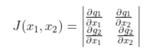
where Jacobian

px 46

and Y1 =g1 (X1, X2) and Y2 =g2 (X1, X2) for some functions g1 and g2 . Here g1 and g2 satisfies the conditions of the Jacobian as continuous and have continuous partial derivatives.

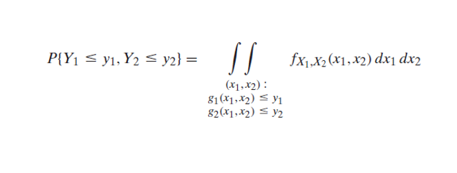
Now the probability for such functions of random variables will be

Image7

Examples on Joint Probability distribution of function of random variables

  1. Find the joint density function of the random variables Y1 =X1 +X2 and Y2=X1 -X2 , where X1 and X2 are the jointly continuous with joint probability density function. also discuss for the different nature of distribution .

Here we first we will check Jacobian

px 47

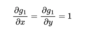
since g1(x1, x2)= x1 + x2  and g2(x1, x2)= x1 – x2 so

px 48

simplifying Y1 =X1 +X2 and Y2=X1 -X2 , for the value of X1 =1/2( Y1 +Y2 ) and X2 = Y1 -Y2 ,

px 49

if these random variables are independent uniform random variables

px 50

or if these random variables are independent exponential random variables with usual parameters

Image10

or if these random variables are independent normal random variables then

px 51
px 52
px 53
  • If X and Y are the independent standard normal variables as given
Conditional distribution

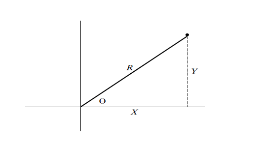
calculate the joint distribution for the respective polar coordinates.

We will convert by usual conversion X and Y into r and θ as

px 54

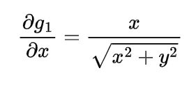
so the partial derivatives of these function will be

px 55
px 56
px 57
px 58

so the Jacobian using this functions is

px 59

if both the random variables X and Y are greater than zero then conditional joint density function is

px 60

now the conversion of cartesian coordinate to the polar coordinate using

px 61

so the probability density function for the positive values will be

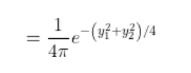
px 62

for the different combinations of X and Y the density functions in similar ways are

px 63
px 64
px 65

now from the average of the above densities we can state the density function as

px 66

and the marginal density function from this joint density of polar coordinates over the interval (0, 2π)

px 67
  • Find the joint density function for the function of random variables

U=X+Y and V=X/(X+Y)

where X and Y are the gamma distribution with parameters (α + λ) and (β +λ) respectively.

Using the definition of gamma distribution and joint distribution function the density function for the random variable X and Y will be

px 68
px 69

consider the given functions as

g1 (x,y) =x+y , g2 (x,y) =x/(x+y),

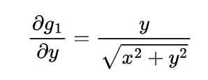
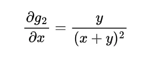
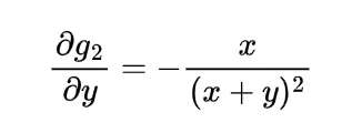
so the differentiation of these function is

px 70
px 71
px 72

now the Jacobian is

px 73

after simplifying the given equations the variables x=uv and y=u(1-v) the probability density function is

px 74
px 75

we can use the relation

px 76
px 77
  • Calculate the joint probability density function for

Y1 =X1 +X2+ X3 , Y2 =X1– X2 , Y3 =X1 – X3

where the random variables X1 , X2, X3 are the standard normal random variables.

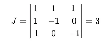
Now let us calculate the Jacobian by using partial derivatives of

Y1 =X1 +X2+ X3 , Y2 =X1– X2 , Y3 =X1 – X3

as

px 78

simplifying for variables X1 , X2 and X3

X1 = (Y1 + Y2 + Y3)/3 , X2 = (Y1 – 2Y2 + Y3)/3 , X3 = (Y1 + Y2 -2 Y3)/3

we can generalize the joint density function as

px 79

so we have

px 80

for the normal variable the  joint probability density function is

px 81

hence

px 82

where the index is

px 83
px 84

compute the joint density function of Y1 ……Yn and marginal density function for Yn where

px 85

and Xi are independent identically distributed exponential random variables with parameter λ.

for the random variables of the form

Y1 =X1 , Y2 =X1 + X2 , ……, Yn =X1 + ……+ Xn

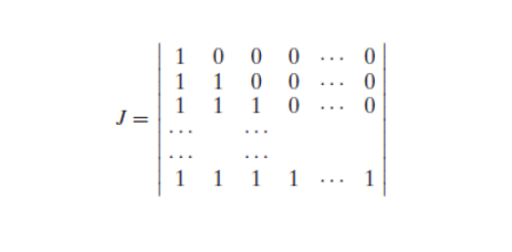
the Jacobian will be of the form

Image11

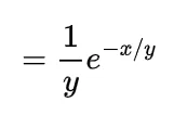
and hence its value is one, and the joint density function for the exponential random variable

px 86

and the values of the variable Xi ‘s will be

px 87

so the joint density function is

px 88
px 89
px 90
px 91

Now to find the marginal density function of Yn we will integrate one by one  as

px 92
px 93

and

px 94 1
px 94 2

like wise

px 96

if we continue this process we will get

px 97

which is the marginal density function.

Conclusion:

The conditional distribution for the discrete and continuous random variable with different examples considering some of the types of these random variables discussed, where the independent random variable plays important role. In addition the  joint distribution for the function of joint continuous random variables also explained with suitable examples, if you require further reading go through below links.

For more post on Mathematics, please refer to our Mathematics Page

Wikipediahttps://en.wikipedia.org/wiki/joint_probability_distribution/” target=”_blank” rel=”noreferrer noopener” class=”rank-math-link”>Wikipedia.org

A first course in probability by Sheldon Ross

Schaum’s Outlines of Probability and Statistics

An introduction to probability and statistics by ROHATGI and SALEH

Jointly Distributed Random Variables: 11 Important Facts

Content

Jointly distributed random variables

     The jointly distributed random variables are the random variable more than one with probability jointly distributed for these random variables, in other words in experiments where the different outcome with their common probability is known as jointly distributed random variable or joint distribution, such type of situation occurs frequently while dealing the problems of the chances.

Joint distribution function | Joint Cumulative probability distribution function | joint probability mass function | joint probability density function

    For the random variables X and Y the distribution function or joint cumulative distribution function is

gif

where the nature of the joint probability depends on the nature of random variables X and Y either discrete or continuous, and the individual distribution functions for X and Y can be obtained using this joint cumulative distribution function as

gif

similarly for Y as

gif

these individual distribution functions of X and Y are known as Marginal distribution functions when joint distribution is under consideration. These distributions are very helpful for getting the probabilities like

and in addition the joint probability mass function for the random variables X and Y is defined as

gif

the individual probability mass or density functions for X and Y can be obtained with the help of such joint probability mass or density function like in terms of discrete random variables as

gif

and in terms of continuous random variable the joint probability density function will be

gif

where C is any two dimensional plane, and the joint distribution function for continuous random variable will be

image 60

the probability density function from this distribution function can be obtained by differentiating

gif

and the marginal probability from the joint probability density function

gif

as

gif

and

gif

with respect to the random variables X and Y respectively

Examples on Joint distribution

  1. The joint probabilities for the random variables X and Y representing the number of mathematics and statistics books from a set of books which contains 3 mathematics, 4 statistics and 5 physics books if 3 books taken randomly
%5Cbinom%7B12%7D%7B3%7D%3D%5Cfrac%7B1%7D%7B220%7D
  • Find the joint probability mass function for the sample of families having 15% no child, 20% 1 child, 35% 2 child and 30% 3 child if the family we choose randomly from this sample for child to be Boy or Girl?

The joint probability we will find by using the definition as

Jointly distributed random variables
Jointly distributed random variables : Example

and this we can illustrate in the tabular form as follows

Jointly distributed random variables
Jointly distributed random variables : Example of joint distribution
  • Calculate the probabilities
gif

if for the random variables X and Y the joint probability density function is given by

gif

with the help of definition of joint probability for continuous random variable

gif

and the given joint density function the first probability for the given range will be

gif
gif
gif
gif

in the similar way the probability

gif
gif
gif
gif

and finally

gif
gif
gif
  • Find the joint density function for the quotient X/Y of random variables X and Y if their joint probability density function is
gif

To find the probability density function for the function X/Y we first find the joint distribution function then we will differentiate the obtained result,

so by the definition of joint distribution function and given probability density function we have

%7BY%7D%28a%29%3DP%20%7B%20%5Cfrac%7BX%7D%7BY%7D%5Cleq%20a%20%7D
gif
gif
gif
gif

thus by differentiating this distribution function with respect to a we will get the density function as

gif

where a is within zero to infinity.

Independent random variables and joint distribution

     In the joint distribution the probability for two random variable X and Y is said to be independent if

gif

where A and B are the real sets. As already in terms of events we know that the independent random variables are the random variables whose events are independent.

Thus for any values of a and b

gif

and the joint distribution or cumulative distribution function for the independent random variables X and Y will be

gif

if we consider the discrete random variables X and Y then

gif

since

gif
gif
gif
gif

similarly for the continuous random variable also

gif

Example of independent joint distribution

  1. If for a specific day in a hospital the patients entered are poisson distributed with parameter λ and probability of male patient as p and probability of female patient as (1-p) then show that the number of male patients and female patients entered in the hospital are independent poisson random variables with parameters λp and λ(1-p) ?

consider the number of male and female patients by random variable X and Y then

gif
gif

as X+Y are the total number of patients entered in the hospital which is poisson distributed so

gif

as the probability of male patient is p and female patient is (1-p) so exactly from total fix number are male or female shows binomial probability as

gif

using these two values we will get the above joint probability as

gif
gif
gif

thus probability of male and female patients will be

gif
gif

and

gif

which shows both of them are poisson random variables with the parameters λp and λ(1-p).

2. find the probability that a person has to wait for more than ten minutes at the meeting for a client as if each client and that person arrives between  12 to 1 pm following uniform distribution.

consider the random variables X and Y to denote the time for that person and client between 12 to 1 so the probability jointly for X and Y will be

image 61
gif
gif
gif
gif

calculate

gif

where X,Y and Z are uniform random variable over the interval (0,1).

here the probability will be

gif

for the uniform distribution the density function

gif

for the given range so

gif
gif
gif
gif

SUMS OF INDEPENDENT RANDOM VARIABLES BY JOINT DISTRIBUTION

  The sum of independent variables X and Y with the probability density functions as continuous random variables, the cumulative distribution function will be

gif
gif
gif
gif

by differentiating this cumulative distribution function for the probability density function of these independent sums are

latex%5Dfty%7D%20F %7BX%7D%20%28a y%29%20f %7BY%7D%28y%29dy
gif
gif

by following these two results we will see some continuous random variables and their sum as independent variables

sum of independent uniform random variables

   for the random variables X and Y uniformly distributed over the interval (0,1) the probability density function for both of these independent variable is

gif

so for the sum X+Y we have

gif

for any value a lies between zero and one

gif

if we restrict a in between one and two it will be

gif

this gives the triangular shape density function

gif

if we generalize for the n independent uniform random variables 1 to n then their distribution function

by mathematical induction will be

gif

sum of independent Gamma random variables

    If we have two independent gamma random variables with their usual density function

gif

then following the density for the sum of independent gamma random variables

gif
gif
gif
gif
gif

this shows the density function for the sum of gamma random variables which are independent

sum of independent exponential random variables

    In the similar way as gamma random variable the sum of independent exponential random variables we can obtain density function and distribution function by just specifically assigning values of gamma random variables.

Sum of independent normal random variable | sum of independent Normal distribution

                If we have n number of independent normal random variables Xi , i=1,2,3,4….n with respective means μi and variances σ2i then their sum is also normal random variable with the mean as Σμi  and variances Σσ2i

    We first show the normally distributed independent sum for two normal random variable X with the parameters 0 and σ2 and Y with the parameters 0 and 1, let us find the probability density function for the sum X+Y with

gif

in the joint distribution density function

gif

with the help of definition of density function of normal distribution

gif
gif

thus the density function will be

gif
gif
gif

which is nothing but the density function of a normal distribution with mean 0 and variance (1+σ2) following the same argument we can say

em%3E%7B2%7D

with usual mean and variances. If we take the expansion and observe the sum is normally distributed with the mean as the sum of the respective means and variance as the sum of the respective variances,

thus in the same way the nth sum will be the normally distributed random variable with the mean as Σμi  and variances Σσ2i

Sums of independent Poisson random variables

If we have two independent Poisson random variables X and Y with parameters λ1 and λ2 then their sum X+Y is also Poisson random variable or Poisson distributed

since X and Y are Poisson distributed and we can write their sum as the union of disjoint events so

gif
gif
em%3E%7B2%7D%5E%7Bn k%7D%7D%7B%28n k%29%21%7D

by using the of probability of independent random variables

em%3E%7B2%7D%5E%7Bn k%7D%7D%7Bk%21%28n k%29%21%7D
em%3E%7B2%7D%5E%7Bn k%7D
em%3E%7B2%7D%29%5E%7Bn%7D

so we get the sum X+Y is also Poisson distributed with the mean λ12

Sums of independent binomial random variables

                If we have two independent binomial random variables X and Y with parameters (n,p) and (m, p) then their sum X+Y is also binomial random variable or Binomial distributed with parameter (n+m, p)

let use the probability of the sum with definition of binomial as

gif
gif
gif
gif
gif

which gives

gif

so the sum X+Y is also binomially distributed with parameter (n+m, p).

Conclusion:

The concept of jointly distributed random variables which gives the distribution comparatively for more than one variable in the situation is discussed in addition the basic concept of independent random variable with the help of joint distribution and sum of independent variables with some example of distribution is given with their parameters, if you require further reading go through mentioned books. For more post on mathematics, please click here.

https://en.wikipedia.org

A first course in probability by Sheldon Ross

Schaum’s Outlines of Probability and Statistics

An introduction to probability and statistics by ROHATGI and SALEH

Gamma Distribution Exponential Family: 21 Important Facts

Content

  1. Special form of Gamma distributions and relationships of Gamma distribution
  2. Gamma distribution exponential family
  3. Relationship between gamma and normal distribution
  4. Poisson gamma distribution | poisson gamma distribution negative binomial
  5. Weibull gamma distribution
  6. Application of gamma distribution in real life | gamma distribution uses | application of gamma distribution in statistics 
  7. Beta gamma distribution | relationship between gamma and beta distribution
  8. Bivariate gamma distribution
  9. Double gamma distribution
  10. Relation between gamma and exponential distribution | exponential and gamma distribution | gamma exponential distribution
  11. Fit gamma distribution
  12. Shifted gamma distribution
  13. Truncated gamma distribution
  14. Survival function of gamma distribution
  15. MLE of gamma distribution | maximum likelihood gamma distribution | likelihood function of gamma distribution
  16. Gamma distribution parameter estimation method of moments | method of moments estimator gamma distribution
  17. Confidence interval for gamma distribution
  18. Gamma distribution conjugate prior for exponential distribution | gamma prior distribution | posterior distribution poisson gamma
  19. Gamma distribution quantile function
  20. Generalized gamma distribution
  21. Beta generalized gamma distribution

Special form of Gamma distributions and relationships of Gamma distribution

  In this article we will discuss the special forms of gamma distributions and the relationships of gamma distribution with different continuous and discrete random variables also some estimation methods  in sampling of population using gamma distribution is briefly discuss.

Gamma distribution exponential family

  The gamma distribution exponential family and it is two parameter exponential family which is largely and applicable family of distribution as most of real life problems can be modelled in the gamma distribution exponential family and the quick and useful calculation  within the exponential family can be done easily, in the two parameter if we take probability density function as

x%7Dx%5E%7B%5Calpha%20

if we restrict the known value of α (alpha) this two parameter family will reduce to one parameter exponential family

x%7D a%20%5C%20%5C%20log%5Clambda%20%5Cfrac%7Bx%5E%7B%5Calpha%20

and for λ (lambda)

gif

Relationship between gamma and normal distribution

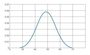
  In the probability density function of gamma distribution if we take alpha nearer to 50 we will get the nature of density function as

Gamma distribution exponential family

even the shape parameter in gamma distribution we are increasing which is resulting in similarity of normal distribution normal curve, if we tend shape parameter alpha tends to infinity the gamma distribution will be more symmetric and normal but as alpha tends to infinity value of x in gamma distribution will tends to minus infinity which result in semi infinite support of gamma distribution infinite hence even gamma distribution becomes symmetric but not same with normal distribution.

poisson gamma distribution | poisson gamma distribution negative binomial

   The poisson gamma distribution and binomial distribution are the discrete random variable whose random variable deals with the discrete values specifically success and failure in the form of Bernoulli trials which gives random success or failure as a result only, now the mixture of Poisson and gamma distribution also known as negative binomial distribution is the outcome of the repeated trial of Bernoulli’s trial, this can be parameterize in different way as if r-th success occurs in number of trials then it can be parameterize as

gif

and if the number of failures before the r-th success then it can be parameterize as

gif

and considering the values of r and p

gif
gif

the general form of the parameterization for the negative binomial or poisson gamma distribution is

gif.latex?P%28X%3Dx%29%3D%5Cbinom%7Bx+r 1%7D%7Bx%7Dp%5E%7Br%7D%281

and alternative one is

gif.latex?P%28X%3Dx%29%3D%5Cbinom%7Bx+r

this binomial distribution is known as negative because of the coefficient

gif.latex?%5Cbinom%7Bx+r 1%7D%7Bx%7D%20%3D%5Cfrac%7B%28x+r 1%29%28x+r 2%29...r%7D%7Bx%21%7D%20%5C%20%3D%20%28 1%29%5E%7Bx%7D%5Cfrac%7B%28 r %28x 1%29%29%28 r %28x 2%29%29...%28 r%29%7D%7Bx%21%7D%20%5C%20%3D%20%28 1%29%5E%7Bx%7D%5Cfrac%7B%28 r%29%28 r 1%29..

and this negative binomial or poisson gamma distribution is well define as the total probability we will get as one for this distribution

gif

The mean and variance for this negative binomial or poisson gamma distribution is

gif
gif

the poisson and gamma relation we can get by the following calculation

%5Cbeta%20%7D%20d%5Clambda
%5Cbeta%20%29%7Dd%5Clambda
gif
gif

Thus negative binomial is the mixture of poisson and gamma distribution and this distribution is used in day to day problems modelling where discrete and continuous mixture we require.

Gamma distribution exponential family

Weibull gamma distribution

   There are generalization of exponential distribution which involve Weibull as well as gamma distribution as the Weibull distribution has the probability density function as

gif

and cumulative distribution function as

gif

where as pdf and cdf of gamma distribution is already we discussed above the main connection between Weibull and gamma distribution is both are generalization of exponential distribution the difference between them is when power of variable is greater than one then Weibull distribution gives quick result while for less than 1 gamma gives quick result.

     We will not discuss here generalized Weibull gamma distribution that require separate discussion.

application of gamma distribution in real life | gamma distribution uses | application of gamma distribution in statistics 

  There are number of  application where gamma distribution is used to model the situation such as insurance claim to aggregate, rainfall amount accumulation, for any product its manufacturing and distribution, the crowd on specific web,  and in telecom exchange etc. actually the gamma distribution give the wait time prediction till next event for nth event. There are number of application of gamma distribution in real life.

beta gamma distribution | relationship between gamma and beta distribution

    The beta distribution is the random variable with the probability density function

gif

where

gif

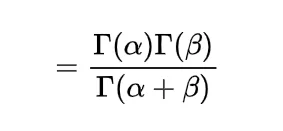
which has the relationship with gamma function as

gif

and beta distribution related to gamma distribution as if X be gamma distribution with parameter alpha and beta as one and Y be the gamma distribution with parameter alpha as one and beta then the random variable X/(X+Y) is beta distribution.

or If X is Gamma(α,1) and Y is Gamma (1, β) then the random variable X/(X+Y) is Beta (α, β) 

and also

gif

bivariate gamma distribution

     A two dimensional or bivariate random variable is continuous if there exists a function f(x,y) such that the joint distribution function

gif

where

gif
gif

and the joint probability density function obtained by

gif

there are number of bivariate gamma distribution one of them is the bivariate gamma distribution with probability density function as

gif

double gamma distribution

  Double gamma distribution is one of the bivariate distribution with gamma random variables having parameter alpha and one with joint probability density function as

em%3E%7B2%7D%29%7Dy %7B1%7D%5E%7B%5Calpha %7B1%7D%20 1%7Dy %7B2%7D%5E%7B%5Calpha %7B2%7D%20 1%7D%20exp%28 y %7B1%7D%20 y %7B2%7D%29%2C%20y %7B1%7D%26gt%3B%200%2C%20y %7B2%7D%26gt%3B%200

this density forms the double gamma distribution with respective random variables and the moment generating function for double gamma distribution is

em%3E%7B2%7D%7D%20%7D

relation between gamma and exponential distribution | exponential and gamma distribution | gamma exponential distribution

   since the exponential distribution is the distribution with the probability density function

and the gamma distribution has the probability density function

clearly the value of alpha if we put as one we will get the exponential distribution, that is the gamma distribution is nothing but the generalization of the exponential distribution, which predict the wait time till the occurrence of next nth event while exponential distribution predict the wait time till the occurrence of the next event.

fit gamma distribution

   As far as fitting the given data in the form of gamma distribution imply finding the two parameter probability density function which involve shape, location and scale parameters so finding these parameters with different application and calculating the mean, variance, standard deviation and moment generating function is the fitting of gamma distribution, since different real life problems will be modelled in gamma distribution so the information as per situation must be fit in gamma distribution for this purpose various technique in various environment is already there e.g in R, Matlab, excel etc.

shifted gamma distribution

     There are as per application and need whenever the requirement of shifting the distribution required from two parameter gamma distribution the new generalized three parameter or any another generalized gamma distribution shift the shape location and scale , such gamma distribution is known as shifted gamma distribution

truncated gamma distribution

     If we restrict the range or domain of the gamma distribution for the shape scale and location parameters the restricted gamma distribution is known as truncated gamma distribution based on the conditions.

survival function of gamma distribution

                The survival function for the gamma distribution is defined the function s(x) as follows

gif

mle of gamma distribution | maximum likelihood gamma distribution | likelihood function of gamma distribution

we know that the maximum likelihood take the sample from the population as a representative and this sample consider as an estimator for the probability density function to maximize for the parameters of density function, before going to gamma distribution recall some basics as for the random variable X the probability density function with theta as parameter has likelihood function as

this we can express as

and method of maximizing this likelihood function can be

if such theta satisfy this equation, and as log is monotone function we can write in terms of log

and such a supremum exists if

em%3E%7Bk%7D%29

now we apply the maximum likelihood for the gamma distribution function as

gif

the log likelihood of the function will be

gif

so is

gif

and hence

gif

This can be achieved also as

gif.latex?%5Ctextbf%7BL%7D%28%5Calpha%20%2C%5Cbeta%20%7C%20x%29%3D%5Cleft%20%28%20%5Cfrac%7B%5Cbeta%20%5E%7B%5Calpha%20%7D%7D%7B%5CGamma%20%28%5Calpha%20%29%7D%20x %7B1%7D%5E%7B%5Calpha%20 1%7D%20e%5E%7B %5Cbeta%20x %7B1%7D%7D%20%5Cright%20%29...%5Cleft%20%28%20%5Cfrac%7B%5Cbeta%20%5E%7B%5Calpha%20%7D%7D%7B%5CGamma%20%28%5Calpha%20%29%7D%20x %7Bn%7D%5E%7B%5Calpha%20 1%7D%20e%5E%7B %5Cbeta%20x %7Bn%7D%7D%20%5Cright%20%29%20%3D%5Cleft%20%28%20%5Cfrac%7B%5Cbeta%20%5E%7B%5Calpha%20%7D%7D%7B%5CGamma%20%28%5Calpha%20%29%7D%20%5Cright%29%5E%7Bn%7D%20%28x %7B1%7D%20%28x %7B2%7D...%28x %7Bn%7D%29%5E%7B%5Calpha%20 1%7D%20e%5E%7B

by

gif

and the parameter can be obtained by differentiating

gif
gif
gif

gamma distribution parameter estimation method of moments | method of moments estimator gamma distribution

   We can calculate the moments of the population and sample with the help of expectation of nth order respectively, the method of moment equates these moments of distribution and sample to estimate the parameters, suppose we have sample of gamma random variable with the probability density function as

gif

we know the first tow moments for this probability density function is

em%3E%7B2%7D%3D%5Cfrac%7B%5Calpha%20%28%5Calpha%20+1%29%20%7D%7B%5Clambda%20%5E%7B2%7D%7D

so

gif

we will get from the second moment if we substitute lambda

em%3E%7B1%7D%5E%7B2%7D%7D%3D%5Cfrac%7B%5Calpha%20+1%7D%7B%5Calpha%20%7D

and from this value of alpha is

em%3E%7B2%7D %5Cmu%20 %7B1%7D%5E%7B2%7D%7D

and now lambda will be

em%3E%7B2%7D %5Cmu%20 %7B1%7D%5E%7B2%7D%7D

and moment estimator using sample will be

gif

confidence interval for gamma distribution

   confidence interval for gamma distribution is the way to estimate the information and its uncertainty which tells the interval is expected to have the true value of the parameter at what percent, this confidence interval is obtained from the observations of random variables, since it is obtained from random it itself is random to get the confidence interval for the gamma distribution there are different techniques in different application that we have to follow.

gamma distribution conjugate prior for exponential distribution | gamma prior distribution | posterior distribution poisson gamma

     The posterior and prior distribution  are the terminologies of Bayesian probability theory and they are conjugate to each other, any two distributions are conjugate if the posterior of one distribution is another distribution, in terms of theta let us show that gamma distribution is conjugate prior to the exponential distribution

if the probability density function of gamma distribution in terms of theta is as

gif

assume the distribution function for theta is exponential from given data

gif

so the joint distribution will be

gif

and using the relation

gif

we have

gif
gif
gif

which is

gif

so gamma distribution is conjugate prior to exponential distribution as posterior is gamma distribution.

gamma distribution quantile function

   Qauntile function of gamma distribution will be the function that gives the points in gamma distribution which relate the rank order of the values in gamma distribution, this require cumulative distribution function and for different language different algorithm and functions for the quantile of gamma distribution.

generalized gamma distribution

    As gamma distribution itself is the generalization of exponential family of distribution adding more parameters to this distribution gives us generalized gamma distribution which is the further generalization of this distribution family, the physical requirements gives different generalization one of the frequent one is using the probability density function as

gif

the cumulative distribution function for such generalized gamma distribution can be obtained by

gif

where the numerator represents the incomplete gamma function as

em%3E%7B0%7D%5E%7B%5Cinfty%7Dt%5E%7Ba 1%7De%5E%7B t%7Ddt

using this incomplete gamma function the survival function for the generalized gamma distribution can be obtained as

gif

another version of this three parameter generalized gamma distribution having probability density function is

gif

where k, β, θ are the parameters greater than zero, these generalization has convergence issues to overcome the Weibull parameters replaces

using this parameterization the convergence of the density function obtained so the more generalization for the gamma distribution with convergence is the distribution with probability density function as

gif.latex?F%28x%29%20%3D%20%5Cbegin%7Bcases%7D%20%5Cfrac%7B%7C%5Clambda%20%7C%7D%7B%5Csigma%20.t%7D.%5Cfrac%7B1%7D%7B%5CGamma%20%5Cleft%20%28%20%5Cfrac%7B1%7D%7B%5Clambda%20%5E%7B2%7D%7D%20%5Cright%20%29%7D.e%5Cleft%20%5B%20%5Cfrac%7B%5Clambda%20.%5Cfrac%7BIn%28t%29 %5Cmu%20%7D%7B%5Csigma%20%7D+In%5Cleft%20%28%20%5Cfrac%7B1%7D%7B%5Clambda%20%5E%7B2%7D%7D%20%5Cright%20%29 e%5E%7B%5Clambda.%5Cfrac%7BIn.%28t%29

Beta generalized gamma distribution

   The gamma distribution involving the parameter beta in the density function because of which sometimes gamma distribution is known as the beta generalized gamma distribution with the density function

gif
gif

with cumulative distribution function as

gif

which is already discussed in detail in the discussion of gamma distribution, the further beta generalized gamma distribution is defined with the cdf as

gif

where B(a,b) is the beta function , and the probability density function for this can be obtained by differentiation and the density function will be

gif

here the G(x) is the above defined cumulative distribution function of gamma distribution, if we put this value then the cumulative distribution function of beta generalized gamma distribution is

%5CGamma%20%28%5Cbeta%20%29%7D%7D%5Comega%20%5E%7Ba 1%7D%20%281 %5Comega%20%29%5E%7Bb 1%7D%20d%5Comega

and the probability density function

gif

the remaining properties can be extended for this beta generalized gamma distribution with usual definitions.

Conclusion:

There are different forms and generalization of gamma distribution and Gamma distribution exponential family as per the real life situations so possible such forms and generalizations were covered in addition with the estimation  methods of gamma distribution in population sampling of information, if you require further reading on Gamma distribution exponential family, please go through below link and books. For more topics on Mathematics please visit our page.

https://en.wikipedia.org/wiki/Gamma_distribution

A first course in probability by Sheldon Ross

Schaum’s Outlines of Probability and Statistics

An introduction to probability and statistics by ROHATGI and SALEH

Inverse Gamma Distribution: 21 Important Facts

Inverse gamma distribution and moment generating function of gamma distribution

      In continuation with gamma distribution we will see the concept of inverse gamma distribution and moment generating function, measure of central tendencies mean, mode and median of gamma distribution by following some of the basic properties of gamma distribution.

gamma distribution properties

Some of the important properties of gamma distribution are enlisted as follows

The probability density function for the gamma distribution is

gif

or

gif

where the gamma function is

gif

2.The cumulative distribution function for the gamma distribution is

gif

where f(x) is the probability density function as given above in particular cdf is

gif

and

gif

respectively or

E[X]=α*β

and

gif
  • The moment generating function M(t) for the gamma distribution is
gif

or

gif
  • The curve for the pdf and cdf is
Inverse gamma distribution
  • The invers gamma distribution can be defined by taking reciprocal of the probability density function of gamma distribution as
gif
  • The sum of independent gamma distribution is again the gamma distribution with sum of the parameters.

inverse gamma distribution | normal inverse gamma distribution

                If in the gamma distribution in the probability density function

or

gif

we take the variable reciprocal or inverse then the probability density function will be

Thus the random variable with this probability density function is known to be the inverse gamma random variable or inverse gamma distribution or inverted gamma distribution.

y%29%5Cleft%20%7C%20%5Cfrac%7B%5Cmathrm%7Bd%7D%20%7D%7B%5Cmathrm%7Bd%7D%20y%7Dy%5E%7B 1%7D%20%5Cright%20%7C
%5Cbeta%20y%29%7Dy%5E%7B 2%7D
y%7D

The above probability density function in any parameter we can take either in the form of lambda or theta the probability density function which is the reciprocal of gamma distribution is the probability density function of inverse gamma distribution.

Cumulative distribution function or cdf of inverse gamma distribution

                The cumulative distribution function for the inverse gamma distribution is the distribution function

gif

in which the f(x) is the probability density function of the inverse gamma distribution as

Mean and variance of the inverse gamma distribution

  The mean and variance of the inverse gamma distribution by following the usual definition of expectation and variance will be

gif

and

gif

Mean and variance of the inverse gamma distribution proof

        To get the mean and variance of the inverse gamma distribution using the probability density function

and the definition of expectations, we first find the expectation for any power of x as

gif
gif.latex?%3D%5Cfrac%7B%5Cbeta%20%5E%7Bn%7D%5Ctau%20%28%5Calpha n%29%7D%7B%28%5Calpha%20 1%29..
gif.latex?%3D%5Cfrac%7B%5Cbeta%20%5E%7Bn%7D%7D%7B%28%5Calpha%20 1%29..

in the above integral we used the density function as

now for the value of α greater than one and n as one

gif

similarly the value for n=2 is for alpha greater than 2

gif

using these expectations will give us the value of variance as

gif

Invers gamma distribution plot | Inverse gamma distribution graph

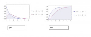
                The inverse gamma distribution is the reciprocal of the gamma distribution so while observing the gamma distribution it is good to observe the nature of the curves of inverse gamma distribution having probability density function as

and the cumulative distribution function by following

gif
Inverse gamma distribution
Inverse gamma distribution graph

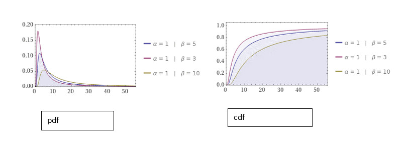
Description: graphs for the probability density function and cumulative distribution function by fixing the value of α as 1 and varying the value of β.

Description: graphs for the probability density function and cumulative distribution function by fixing the value of α as 2 and varying the value of β

Description: graphs for the probability density function and cumulative distribution function by fixing the value of α as 3 and varying the value of β.

Description: graphs for the probability density function and cumulative distribution function by fixing the value of β as 1 and varying the value of α.

Description: graphs for the probability density function and cumulative distribution function by fixing the value of β as 2 and varying the value of α

Description: graphs for the probability density function and cumulative distribution function by fixing the value of β as 3 and varying the value of α.

moment generating function of gamma distribution

Before understanding the concept of moment generating function for the gamma distribution let us recall some concept of moment generating function

Moments

    The moment of the random variable is defined with the help of expectation as

gif

this is known as r-th moment of the random variable X it is the moment about origin and commonly known as raw moment.

     If we take the r-th moment of the random variable about the mean μ as

gif

this moment about the mean is known as central moment and the expectation will be as per the nature of random variable as

gif
gif

in the central moment if we put values of r then we get some initial moments as

em%3E%7B1%7D%3D0%20%2C%20%7B%5Cmu%7D %7B2%7D%3D%5Csigma%20%5E%7B2%7D

If we take the binomial expansion in the central moments then we can easily get the relationship between the central and raw moments as

em%3E%7Br j%7D%7B%5Cmu%7D%5E%7Bj%7D%20+%20..

some of the initial relationships are as follows

Moment generating function

   The moments we can generate with the help of a function that function is known as moment generating function and is defined as

gif

this function generates the moments with the help of expansion of exponential function in either of the form

gif

using Taylors form as

em%3E%7Br%7D%5Cfrac%7Bt%5E%7Br%7D%7D%7Br%21%7D+.

differentiating this expanded function with respect to t gives the different moments as

em%3E%7BX%7D%28t%29%5Clvert %7Bt%3D0%20%7D

on in another way if we take the derivative directly as

gif

since for both discrete

gif

and continuous we have

gif

so for t=0 we will get

gif

likewise

gif

as

gif

and in general

gif

there is two important relations for the moment generating functions

b%29%20%5C%20M %7B%28X+Y%29%7D%28t%29%3DM %7BX%7D%28t%29%20M %7BY%7D%28t%29

moment generating function of a gamma distribution | mgf of gamma distribution | moment generating function for gamma distribution

Now for the gamma distribution the moment generating function M(t) for the pdf

is

gif

and for the pdf

the moment generating function is

gif

gamma distribution moment generating function proof | mgf of gamma distribution proof

    Now first take the form of probability density function as

and using the definition of moment generating function M(t) we have

gif
gif

we can find the mean and variance of the gamma distribution with the help of moment generating function as differentiating with respect to t two times this function we will get

gif

if we put t=0 then first value will be

gif

and

gif

Now putting the value of these expectation in

gif

alternately for the pdf of the form

gif

the moment generating function will be

%5Cbeta%20%29%7D%20x%5E%7B%5Calpha%20 1%7D%20dx%20%5C%20%3D%20%5Cleft%20%28%20%5Cfrac%7B1%7D%7B1 %5Cbeta%20t%7D%20%5Cright%20%29%5E%7B%5Calpha%20%7D%5Cint %7B0%7D%5E%7B%5Cinfty%7D%20%5Cfrac%7By%5E%7B%5Calpha%20 1%7D%20e%5E%7B y%7D%7D%7B%5Ctau%20%28%5Calpha%20%29%7D%20dy%20%5C%20%5C%20%2C%20%5C%20%5C%20t%26lt%3B%20%5Cfrac%7B1%7D%7B%5Cbeta%20%7D%20%5C%20%3D%20%281 %5Cbeta%20t%29%5E%7B %5Calpha%20%7D%20%5C%20%5C%20t%26lt%3B%20%5Cfrac%7B1%7D%7B%5Cbeta%20%7D

and differentiating and putting t=0 will give mean and variance as follows

gif

2nd moment of gamma distribution

   The second moment of gamma distribution by differentiating moment generating function two times and putting the value of t=0 in second derivative of that function we will get

gif

third moment of gamma distribution

                The third moment of gamma distribution we can find by differentiating the moment generating function three times and putting the value of t=0 in third derivative of the mgf we will get

gif

or directly by integrating as

gif

 sigma for gamma distribution

   sigma or standard deviation of gamma distribution we can find by taking the square root of variance of gamma distribution of type

gif

or

gif

for any defined value of alpha, beta and lambda.

characteristic function of gamma distribution | gamma distribution characteristic function

      If the variable t in the moment generating function is purely an imaginary number as t=iω then the function is known as the characteristic function of gamma distribution denoted and expressed as

gif

as for any random variable the characteristic function will be

gif

Thus for the gamma distribution the characteristic function by following the pdf of gamma distribution is

gif

following

%5Cbeta%20%29%5E%7B %5Calpha%20%7D%5Cint %7B0%7D%5E%7B%5Cinfty%7Dx%5E%7B%5Calpha%20 1%7De%5E%7B x%7D%20dx%3D%5Ctau%20%28%5Calpha%20%29%5Cbeta%20%5E%7B%5Calpha%20%7D%281 i%5Cbeta%20t%29%5E%7B %5Calpha%20%7D

There is another form of this characteristics function also if

2%7D

then

2%7D

sum of gamma distributions | sum of exponential distribution gamma

  To know the result of sum of gamma distribution we must first of all understand sum of independent random variable for the continuous random variable, for this let us have probability density functions for the continuous random variables X and Y then the cumulative distribution function for the sum of random variables will be

gif

differentiating this convolution of integral for the probability density functions of X and Y will give the probability density function for the sum of random variables as

em%3E%7B %5Cinfty%7D%5E%7B%5Cinfty%7DF %7BX%7D%28a y%29f %7BY%7D%28y%29%20dy%20%5C%20%3D%20%5Cint %7B %5Cinfty%7D%5E%7B%5Cinfty%7D%5Cfrac%7B%5Cmathrm%7Bd%7D%20%7D%7B%5Cmathrm%7Bd%7D%20a%7DF %7BX%7D%28a y%29f %7BY%7D%28y%29%20dy%20%5C%20%3D%20%5Cint %7B %5Cinfty%7D%5E%7B%5Cinfty%7Df %7BX%7D%28a y%29f %7BY%7D%28y%29%20dy

Now let us prove if X and Y are the gamma random variables with respective density functions then there sum will also be gamma distribution with sum of same parameters

considering the probability density function of the form

for the random variable X take alpha as  s and for random variable Y take alpha as t so using the probability density for the sum of random variables we have

em%3E%7B0%7D%5E%7Ba%7D%5Clambda%20e%5E%7B %5Clambda%20%28a y%29%7D%20%28%5Clambda%20%28a y%29%29%5E%7Bs 1%7D%5Clambda%20e%5E%7B %5Clambda%20y%7D%20%28%5Clambda%20y%29%5E%7Bt 1%7D%20dy

here C is independent of a , now the value will be

gif

which represent the probability density function of sum of X and Y and which is of the Gamma distribution, hence the sum of the gamma distribution also represents the gamma distribution by respective sum of parameters.

mode of gamma distribution

    To find the mode of gamma distribution let us consider the probability density function as

now differentiate this pdf with respect to x, we will get the differentiation as

gif

this will be zero for x=0 or x=(α -1)/λ

so these are only critical points at which our first derivative will be zero if alpha greater than or equal to zero then x=0 will not be mode because this makes pdf zero so mode will be (α -1)/λ

and for alpha strictly less than one the derivative decreases from infinity to zero as x increases from zero to infinity so this is not possible hence the mode of gamma distribution is

gif

median of gamma distribution

The median of the gamma distribution can be found with the help of inverse gamma distribution as

gif

or

gif

provided

gif

which gives

gif.latex?median%28n%29%3Dn+%5Cfrac%7B2%7D%7B3%7D+%5Cfrac%7B8%7D%7B405n%7D%20 %5Cfrac%7B64%7D%7B5103n%5E%7B2%7D%7D+..

gamma distribution shape

     Gamma distribution takes different shape depending on the shape parameter when shape parameter is one gamma distribution is equal to the exponential distribution but when we vary the shape parameter the skewness of the curve of gamma distribution decreases as the increase in the shape parameter, in another words the shape of the curve of gamma distribution changes as per the standard deviation .

skewness of gamma distribution

    skewness of any distribution can be observed by observing the probability density function of that distribution and skewness coefficient

em%3E%7B3%7D%7D%7B%5Csigma%20%5E%7B3%7D%7D

for the gamma distribution we have

gif.latex?E%28X%5E%7Bk%7D%29%3D%5Cfrac%7B%28%5Calpha%20+k 1%29%28%5Calpha%20+k 2%29..

so

gif

this shows the skewness depends on alpha only if alpha increases to infinity curve will be more symmetric and sharp and when alpha goes to zero the gamma distribution density curve positively skewed which can be observed in the density graphs.

generalized gamma distribution | shape and scale parameter in gamma distribution | three parameter gamma distribution | multivariate gamma distribution

gif

where γ, μ and β are the shape, location and scale parameters respectively, by assigning specific values to these parameters we can get the two parameter gamma distribution specifically if we put μ=0, β=1 then we will get standard gamma distribution as

gif

using this 3 parameter gamma distribution probability density function we can find the expectation and variance by following there definition respectively.

Conclusion:

The concept of reciprocal of gamma distribution that is inverse gamma distribution in comparison with gamma distribution and measure of central tendencies of gamma distribution with the help of moment generating function were the focus of this article, if you require further reading go through suggested books and links. For more post on mathematics, visit our mathematics page.

https://en.wikipedia.org/wiki/Gamma_distribution

A first course in probability by Sheldon Ross

Schaum’s Outlines of Probability and Statistics

An introduction to probability and statistics by ROHATGI and SALEH

Gamma Distribution: 7 Important Properties You Should Know

Gamma Distribution

One of the continuous random variable and continuous distribution is the Gamma distribution, As we know the continuous random variable deals with the continuous values or intervals so is the Gamma distribution with specific probability density function and probability mass function, in the successive discussion we discuss in detail the concept, properties and results with examples of gamma random variable and gamma distribution.

Gamma random variable or Gamma distribution | what is gamma distribution | define gamma distribution | gamma distribution density function | gamma distribution probability density function | gamma distribution proof

A continuous random variable with probability density function

gif

is known to be Gamma random variable or Gamma distribution where the α>0, λ>0 and the gamma function

gif

we have the very frequent property of gamma function by integration by parts as

gif
gif
gif

If we continue the process starting from n then

gif
gif
gif.latex?%3D%28n 1%29%20%28n 2%29....3.

and lastly the value of gamma of one will be

CodeCogsEqn

thus the value will be

gif

cdf of gamma distribution | cumulative gamma distribution | integration of gamma distribution

The cumulative distribution function(cdf) of gamma random variable or simply the distribution function of gamma random variable is same as that of continuous random variable provided the probability density function is different i.e

gif

here the probability density function is as defined above for the gamma distribution, the cumulative distribution function we can write also as

gif

in both of the above formats the value of pdf is as follows

gif

where the α >0, λ>0 are real numbers.

Gamma distribution formula | formula for gamma distribution | gamma distribution equation | gamma distribution derivation

To find the probability for the gamma random variable the probability density function we have to use for different given α >0 , λ >0 is as

gif


and using the above pdf the distribution for the gamma random variable we can obtain by

gif

Thus the gamma distribution formula require the pdf value and the limits for the gamma random variable as per the requirement.

Gamma distribution example


show that the total probability for the gamma distribution is one with the given probability density function i.e

gif

for λ >0, α>0.
Solution:
using the formula for the gamma distribution

gif
gif

since the probability density function for the gamma distribution is

gif


which is zero for all the value less than zero so the probability will be now

gif
gif

using the definition of gamma function

gif

and substitution we get

gif

thus

gif

Gamma distribution mean and variance | expectation and variance of gamma distribution | expected value and variance of gamma distribution | Mean of gamma distribution | expected value of gamma distribution | expectation of gamma distribution


In the following discussion we will find the mean and variance for the gamma distribution with the help of standard definitions of expectation and variance of continuous random variables,

The expected value or mean of the continuous random variable X with probability density function

gif

or Gamma random variable X will be

gif

mean of gamma distribution proof | expected value of gamma distribution proof

To obtain the expected value or mean of gamma distribution we will follow the gamma function definition and property,
first by the definition of expectation of continuous random variable and probability density function of gamma random variable we have

gif
gif
gif

by cancelling the common factor and using the definition of gamma function

gif

now as we have the property of gamma function

gif

the value of expectation will be

gif

thus the mean or expected value of gamma random variable or gamma distribution we get is

gif

variance of gamma distribution | variance of a gamma distribution

The variance for the gamma random variable with the given probability density function

gif

or variance of the gamma distribution will be

gif

variance of gamma distribution proof


As we know that the variance is the difference of the expected values as

gif

for the gamma distribution we already have the value of mean

gif

now first let us calculate the value of E[X2], so by definition of expectation for the continuous random variable we have
since the function f(x) is the probability distribution function of gamma distribution as

gif

so the integral will be from zero to infinity only

gif
gif

so by definition of the gamma function we can write

gif
gif

Thus using the property of the gamma function we got the value as

gif


Now putting the value of these expectation in

gif
gif
gif

thus, the value of variance of gamma distribution or gamma random variable is

gif

Gamma distribution parameters | two parameter gamma distribution | 2 variable gamma distribution


The Gamma distribution with the parameters λ>0, α>0 and the probability density function

gif

has statistical parameters mean and variance as

gif

and

gif

since λ is positive real number, to simplify and easy handling another way is to set λ=1/β so this gives the probability density function in the form

gif

in brief the distribution function or cumulative distribution function for this density we can express as

this gamma density function gives the mean and variance as

gif

and

gif


which is obvious by the substitution.
Both the way are commonly used either the gamma distribution with the parameter α and λ denoted by gamma (α, λ) or the gamma distribution with the parameters β and λ denoted by gamma (β, λ) with the respective statistical parameters mean and variance in each of the form.
Both are nothing but the same.

Gamma distribution plot | gamma distribution graph| gamma distribution histogram

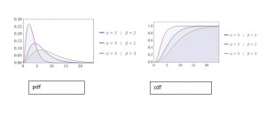
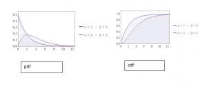
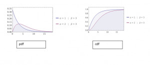
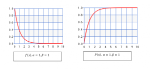
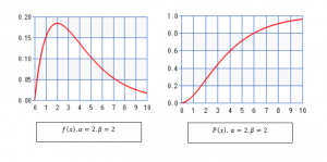
The nature of the gamma distribution we can easily visualize with the help of graph for some of specific values of the parameters, here we draw the plots for the probability density function and cumulative density function for some values of parameters
let us take probability density function as

gif

then cumulative distribution function will be

gamma distribution

Description: graphs for the probability density function and cumulative distribution function by fixing the value of alpha as 1 and varying the value of beta.

gamma distribution

Description: graphs for the probability density function and cumulative distribution function by fixing the value of alpha as 2 and varying the value of beta

gamma distribution

Description: graphs for the probability density function and cumulative distribution function by fixing the value of alpha as 3 and varying the value of beta

gamma distribution

Description: graphs for the probability density function and cumulative distribution function by fixing the value of beta  as 1 and varying the value of alpha

gamma distribution

Description: graphs for the probability density function and cumulative distribution function by fixing the value of beta  as 2 and varying the value of alpha

gamma distribution

Description: graphs for the probability density function and cumulative distribution function by fixing the value of beta as 3 and varying the value of alpha.

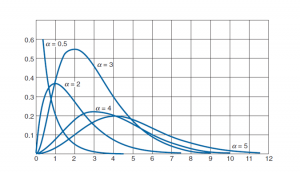
In general different curves as for alpha varying is

Gamma distribution
Gamma distribution graph

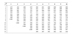
Gamma distribution table | standard gamma distribution table


The numerical value of gamma function

gif


known as incomplete gamma function numerical values as follows

Gamma distribution


The gamma distribution numerical value for sketching the plot for the probability density function and cumulative distribution function for some initial values are as follows

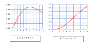
1xf(x),α=1,β=1f(x),α=2,β=2f(x),α=3,β=3P(x),α=1,β=1P(x),α=2,β=2P(x),α=3,β=3
0100000
0.10.9048374180.023780735611.791140927E-40.095162581960.0012091042746.020557215E-6
0.20.81873075310.04524187096.929681371E-40.18126924690.004678840164.697822176E-5
0.30.74081822070.064553098230.0015080623630.25918177930.010185827111.546530703E-4
0.40.6703200460.081873075310.002593106130.3296799540.017523096313.575866931E-4
0.50.60653065970.097350097880.0039188968750.39346934030.026499021166.812970042E-4
0.60.54881163610.11112273310.0054582050210.45118836390.036936313110.001148481245
0.70.49658530380.12332041570.0071856645830.50341469620.048671078880.001779207768
0.80.44932896410.13406400920.0090776691950.55067103590.061551935550.002591097152
0.90.40656965970.14346633410.011112273310.59343034030.075439180150.003599493183
10.36787944120.15163266490.013269098340.63212055880.090204010430.004817624203
1.10.33287108370.15866119790.015529243520.66712891630.10572779390.006256755309
1.20.30119421190.16464349080.017875201230.69880578810.12190138220.007926331867
1.30.2725317930.16966487750.02029077660.7274682070.13862446830.00983411477
1.40.24659696390.17380485630.022761011240.75340303610.15580498360.01198630787
1.50.22313016010.17713745730.025272110820.77686983990.17335853270.01438767797
1.60.2018965180.17973158570.027811376330.7981034820.19120786460.01704166775
1.70.18268352410.18165134610.030367138940.81731647590.20928237590.01995050206
1.80.16529888820.18295634690.032928698170.83470111180.22751764650.02311528775
1.90.14956861920.18370198610.035486263270.85043138080.24585500430.02653610761
20.13533528320.18393972060.038030897710.86466471680.26424111770.03021210849
2.10.12245642830.18371731830.040554466480.87754357170.28262761430.03414158413
2.20.11080315840.1830790960.043049586250.88919684160.30097072420.03832205271
2.30.10025884370.18206614240.045509578110.89974115630.31923094580.04275032971
2.40.090717953290.18071652720.047928422840.90928204670.33737273380.04742259607
2.50.082084998620.1790654980.050300718580.91791500140.35536420710.052334462
2.60.074273578210.17714566550.052621640730.92572642180.3731768760.05748102674
2.70.067205512740.17498717590.054886904070.93279448730.39078538750.0628569343
2.80.060810062630.17261787480.057092726880.93918993740.40816728650.06845642568
2.90.055023220060.17006345890.059235797090.94497677990.42530279420.07427338744
30.049787068370.16734762010.06131324020.95021293160.44217459960.08030139707
Image9
Gamma Distribution Graph
Image10
Image11

finding alpha and beta for gamma distribution | how to calculate alpha and beta for gamma distribution | gamma distribution parameter estimation


For a gamma distribution finding alpha and beta we will take mean and variance of the gamma distribution

gif

and

gif


now we will get value of beta as

gif


so

gif


and

gif

thus

gif

only taking some fractions from the gamma distribution we will get the value of alpha and beta.

gamma distribution problems and solutions | gamma distribution example problems | gamma distribution tutorial | gamma distribution question

1. Consider the time require to resolve the problem for a customer is gamma distributed in hours with the mean 1.5 and variance 0.75 what would be the probability that the problem resolving time exceed 2 hours, if time exceeds 2 hours what would be the probability that the problem will resolved in at least 5 hours.

solution: since the random variable is gamma distributed with mean 1.5 and variance 0.75 so we can find the values of alpha and beta and with the help of these values the probability will be

P(X>2)=13e-4=0.2381

and

P(X>5 | X>2)=(61/13)e-6=0.011631

2. If the negative feedback in week from the users is modelled in gamma distribution with parameters alpha 2 and beta as 4 after the 12 week negative feedback came after restructuring the quality, from this information can restructuring improves the performance ?

solution: As this is modelled in gamma distribution with α=2, β=4

we will find the mean and standard deviation as μ =E(x)=α * β=4 * 2=8

since the value X=12 is within the standard deviation from the mean so we can not say this is improvement or not by the restructuring the quality, to prove the improvement caused by the restructuring information given is insufficient.

3. Let X be the gamma distribution with parameters α=1/2, λ=1/2 , find the probability density function for the function Y=Square root of X

Solution: let us calculate the cumulative distribution function for Y as

2%7D

now differentiating this with respect to y gives the probability density function for Y as

2%7D

and the range for y will be from 0 to infinity


Conclusion:

The concept of gamma distribution in probability and statistic is the one of the important day to day applicable distribution of exponential family, all the basic to higher level concept were discussed so far related to gamma distribution, if you require further reading, please go through mentioned books. You can also visit out mathematics page for more Topic

https://en.wikipedia.org/wiki/Gamma_distribution
A first course in probability by Sheldon Ross
Schaum’s Outlines of Probability and Statistics
An introduction to probability and statistics by ROHATGI and SALEH

Probability Theory: 9 Facts You Should Know

Image1 1 300x179 1

A brief Description of Probability theory

In the previous articles, the probability we discussed was at very basic level, Probability is a means of expressing information that an occurrence of an event has occurred, In pure mathematics the concept of probability has been described in the form of probability theory which is widely used in the areas of real life as well as different branches of philosophy, science, gambling, finance, statistics and mathematics etc. for finding the likelihood of main events.

    Probability theory is the branch of mathematics which deals with the random experiment and its outcome, the core objects for dealing such analysis of the random experiment are events, random variable, stochastic processes, non-deterministic events etc.

Providing an example when we toss a coin or die this event although is random but when we repeat such trial number of times the result of such trial or event will result in a particular statistical arrangement which we can predict after studying via law of large numbers or the central limit theorems etc. so likewise we can use probability theory for the day to day activity of human beings e.g. large set of data can be analyze by quantitative analysis, for  explanation of those systems for which we have insufficient information we can use probability theory e.g. complex systems in statistical mechanics, for physical phenomena of atomic scales in quantum mechanics. 

    There are number of real life situations as well as applications where the probabilistic situation occurs the probability theory will be used provided the familiarity of the concept and the handling of the results and relations of probability theory.  In following we will get some differentiation of the situations with the help of some terms in probability theory.     

Discrete probability

Discrete probability theory is the study of random experiments in which the result can be counted numerically, so here the restriction is the events whatever occurred must be countable subset of given sample space. It includes the experiment of throwing coin or dice, random walk, picking cards from deck, balls in bags etc.

Continuous probability

Continuous probability theory is the study of random experiments in which the result is within the continuous intervals, so here restriction is the events whatever occurred must be in the form of continuous intervals as a subset of sample space.

Measure-theoretic probability

The Measure theoretic probability theory deals with the any of discrete and continuous random outcome, and differentiate in which situation what measure have to be used. The measure theoretic probability theory also deals with the probability distributions which is neither discrete nor continuous nor the mixture of both.

     So to study the probability we must know first of all what is the nature of random experiment either that is discrete, continuous or mixture of both or neither, depending on this we can set our strategies which way we have to follow.  we will discuss all the situation consecutively one by one.

EXPERIMENT

Any action that produces a result or an outcome is called as experiment. There are two types of experiment.

Deterministic Experiments  Non-deterministic Experiments (or Random Experiments)
Any experiment whose outcome we can predict in advance under some conditions.Any experiment whose outcome or result we cannot able to predict in advance.
For example flow of current in specific circuit based on the power provided we know by some physical laws.For example tossing of an unbiased coin we don’t know head will come or tail
We don’t need probability theory for such experiments outcome.We need probability theory for such experiments outcome.

Theory of Probability is basically depending on the model of a random experiment, that implies an experiment whose outcome is unpredictable with certainty, before the experiment is run. People normally thinks that the experiment can be recurrent forever under fundamentally the same circumstances.   

   This presumption is important because the theory of Probability is concerned with the long-term practices as the experiment is recreated. Naturally, a proper definition of a random experiment needs a careful definition of specifically what information about the experiment is being recorded, that is, a careful definition of what constitutes an outcome.

SAMPLE SPACE

As already discussed Sample space is nothing but the set having all possible outcomes of non-deterministic or random experiment. In mathematical analysis random variable which is outcome of such experiment is a real valued function denoted by X i.e X:A ⊆ S → ℝ  that we will discuss in detail later.  Here also we can categorize sample space as finite or infinite.  Infinite sample spaces can be discrete or continuous.

Finite Sample Spaces  Infinite Discrete Sample Spaces  
Tossing a coin or anything with two different result {H, T}Repeatedly tossing a coin until first head shows possible outcome may be {H,TH,TTH,TTTH,…………}
Throwing a die {1, 2, 3, 4, 5, 6}Throwing a die repeatedly till 6 come
Drawing a card from a deck of 52 cardsDrawing a card and replacing till queen come
Choosing a birthday from a year {1, 2, 3, 4, …, 365}.Arriving time of two consecutive trains

EVENT

Event as already we know is subset of the sample space of random experiment for which we are discussing the probability.  In other word we can say any element in the power set of sample space for finite sample space is Event and for infinite we have to exclude some subsets.

Independent eventsDependent Events
If there is no effect of the events to other eventsOccurrence of one event affect other events
For example tossing a coinDrawing a card without returning.
Probabilities of the events also not affectedProbabilities of the events affected
P(A ⋂ B) = P (A) X P(B)P(A ⋂ B) =P(A) X P(B/A)
P(B/A) is the conditional prob. of B given A

RANDOM VARIABLE

The understanding of random variable is very important for the study of probability theory. Random variable  is very helpful to generalized the concept of probability which gives mathematical property to probabilities questions  and the use of measure theoretic probability is based on random variable.  Random variable which is outcome of random experiment is a real valued function denoted by X i.e X:A ⊆ S → ℝ

Discrete Random VariableContinuous Random Variable
Countable outcome of random experimentOutcome of random experiment in range
For a coin toss, the possible events are heads or tails. so random variable takes the values :
X=1 if heads and X=0 if tails
a real number between zero and one
For throwing a die X=1,2,3,4,5,6For the time of travelling X=(3,4)

A random variable can be thought of as an unknown value that may change every time it is inspected. Thus, a random variable can be thought of as a function mapping the sample space of a random process to the real numbers.

Probability Distributions

Probability distribution is defined as the collection of random variable with its probability,

so obviously depending on the nature of random variable we can categorize as

Discrete Probability DistributionContinuous Probability Distribution
If random variable is discrete then probability distribution is known as discrete probability distributionIf random variable is continuous then probability distribution is known as continuous probability distribution
For example number of tails for tossing a coin two times  can be distributed as result will be TT,HH,TH,HT
X(no of tails): 0 1 2
P(x) : 1/4 1/2 1/3
A continuous probability distribution differs from a discrete probability distribution so for the random variable X ≤ a its probability P(X ≤ a) can be considered as the area under the curve (See the below image)
continuous probability distribution

      In the similar way for dealing with probability of random variable depends on the nature of random variable, so the concepts we are using will depend on the nature of random variable.

Conclusion:

   In this article we mainly discuss the scenario of probability, how we can deal the probability and some concept comparatively. Before discussing the core subject this discussion is important so that the problems we deal stands where we know clearly. In the consecutive articles we relate probability to random variable and some familiar terms related to probability theory we will discuss, if you want further reading then go through:

Schaum’s Outlines of Probability and Statistics

https://en.wikipedia.org/wiki/Probability

For more topics on mathematics please check this page.

Normal Random Variable : 3 Important Facts

01

Normal Random variable and Normal distribution

      The random variable with uncountable set of values is known to be continuous random variable, and the probability density function with the help of integration as area under the curve gives the continuous distribution, Now we will focus one of the most used and frequent continuous random variable viz normal random variable which has another name as Gaussian random variable or Gaussian distribution.

Normal random variable

      Normal random variable is the continuous random variable with probability density function

01

having mean μ and variance σ2 as the statistical parameters and geometrically the probability density function has the bell shaped curve which is symmetric about the mean μ.

Normal Random variable

We know that probability density function has the total probability as one so

02

by putting y= (x-μ)/σ

03
04
05
06
07

this double integration can be solved by converting it  into polar form

08

which is the required value so it is verified for the integral I.

  • If X is normally distributed with parameter μ  and σ2 then Y=aX+b is also normally distributed with the parameters  aμ+b and a2μ2

Expectation and Variance of Normal Random variable

The Expected value of the normal random variable and the variance we will get with the help of

09

where X is normally distributed with the parameters mean μ and standard deviation σ.

10

since mean of Z is zero so we have the variance as

11

by using integration by parts

12 1

for the variable Z the graphical interpretation is as follows

Normal Random variable

and the area under the curve for this variable Z which is known as standard normal variable, it is calculated for the reference (given in the table), as the curve is symmetric so for negative value the area will be same as that of positive values

13
z0.000.010.020.030.040.050.060.070.080.09
0.00.500000.503990.507980.511970.515950.519940.523920.527900.531880.53586
0.10.539830.543800.547760.551720.555670.559620.563560.567490.571420.57535
0.20.579260.583170.587060.590950.594830.598710.602570.606420.610260.61409
0.30.617910.621720.625520.629300.633070.636830.640580.644310.648030.65173
0.40.655420.659100.662760.666400.670030.673640.677240.680820.684390.68793
0.50.691460.694970.698470.701940.705400.708840.712260.715660.719040.72240
0.60.725750.729070.732370.735650.738910.742150.745370.748570.751750.75490
0.70.758040.761150.764240.767300.770350.773370.776370.779350.782300.78524
0.80.788140.791030.793890.796730.799550.802340.805110.807850.810570.81327
0.90.815940.818590.821210.823810.826390.828940.831470.833980.836460.83891
1.00.841340.843750.846140.848490.850830.853140.855430.857690.859930.86214
1.10.864330.866500.868640.870760.872860.874930.876980.879000.881000.88298
1.20.884930.886860.888770.890650.892510.894350.896170.897960.899730.90147
1.30.903200.904900.906580.908240.909880.911490.913080.914660.916210.91774
1.40.919240.920730.922200.923640.925070.926470.927850.929220.930560.93189
1.50.933190.934480.935740.936990.938220.939430.940620.941790.942950.94408
1.60.945200.946300.947380.948450.949500.950530.951540.952540.953520.95449
1.70.955430.956370.957280.958180.959070.959940.960800.961640.962460.96327
1.80.964070.964850.965620.966380.967120.967840.968560.969260.969950.97062
1.90.971280.971930.972570.973200.973810.974410.975000.975580.976150.97670
2.00.977250.977780.978310.978820.979320.979820.980300.980770.981240.98169
2.10.982140.982570.983000.983410.983820.984220.984610.985000.985370.98574
2.20.986100.986450.986790.987130.987450.987780.988090.988400.988700.98899
2.30.989280.989560.989830.990100.990360.990610.990860.991110.991340.99158
2.40.991800.992020.992240.992450.992660.992860.993050.993240.993430.99361
2.50.993790.993960.994130.994300.994460.994610.994770.994920.995060.99520
2.60.995340.995470.995600.995730.995850.995980.996090.996210.996320.99643
2.70.996530.996640.996740.996830.996930.997020.997110.997200.997280.99736
2.80.997440.997520.997600.997670.997740.997810.997880.997950.998010.99807
2.90.998130.998190.998250.998310.998360.998410.998460.998510.998560.99861
3.00.998650.998690.998740.998780.998820.998860.998890.998930.998960.99900
3.10.999030.999060.999100.999130.999160.999180.999210.999240.999260.99929
3.20.999310.999340.999360.999380.999400.999420.999440.999460.999480.99950
3.30.999520.999530.999550.999570.999580.999600.999610.999620.999640.99965
3.40.999660.999680.999690.999700.999710.999720.999730.999740.999750.99976
3.50.999770.999780.999780.999790.999800.999810.999810.999820.999830.99983

since we have used the substitution

14

Here keep in mind that Z is standard normal variate where as continuous random variable X is normally distributed normal random variable with mean μ and standard deviation σ.

So to find the distribution function for the random variable we will use the conversion to the standard normal variate as

16

for any value of a.

Example: In the standard normal curve find the area between the points 0 and 1.2.

If we follow the table the value of 1.2 under the column 0 is 0.88493 and value of 0 is 0.5000 ,

Normal Random variable
17

Example: find the area for the standard normal curve within -0.46 to 2.21.

Normal Random variable

From the shaded region we can bifurcate this region from -0.46 to 0 and 0 to 2.21 because the normal curve is symmetric about y axis so the area from -0.46 to 0 is same as the are from 0 to 0.46 thus from the table

18

and

19

so we can write it as

Total Area =(area between z = -0.46 and z=0 ) + (area between z =0 and z=2.21)

= 0.1722 + 0.4864

= 0.6586

Example: If X is normal random variable with mean 3 and variance 9 then find the following probabilities

P2<X<5

P{X>0}

P|X-3|>6

Solution:  since we have

20
21.PNG
22
Normal Random variable

so bifurcating into the intervals -1/3 to 0 and 0 to 2/3 we will get the solution from the tabular values

23

or

24
25

=0.74537 -1 + 0.62930 =0.37467

and

26
Normal Random variable
27.PNG
Normal Random variable

Example: An observer in paternity case states that the length (in days) of human growth

is normally distributed with parameters mean  270 and variance 100. In this case the suspect  who is father of the child provided the proof that he was out of the country during a period that started 290 days before the birth of the child and ended 240 days earlier the birth. Find the probability that the mother could have had the very long or very short pregnancy indicated by the witness?

Let X denote the normally distributed random variable for gestation and consider the suspect is the father of the child. In that case the birth of the child happened within the specified time has the probability

29

Relation between Normal random variable and Binomial random variable

      In case of Binomial distribution the mean is np and the variance is npq so if we convert such binomial random variable with such  mean and standard deviation having n very large and p or q are very small going nearer to zero then standard normal variable Z with the help of these mean and variance is

30.PNG

here in terms of Bernouli trials X considers the number of successes in n trials. As n is increases and goes nearer to infinity this normal variate goes in the same way to become standard normal variate.

The relation of binomial and standard normal variate we can find with the help of following theorem.

DeMoivre Laplace limit theorem

If Sn denotes the number of successes that occur when n  independent trials, each resulting in a success with probability p , are performed, then, for any a < b ,

31.PNG
32

Example: With the help of normal approximation to the binomial random variable find the probability of occurrence of 20 times tail when a fair coin tossed 40 times.

Solution: Suppose the random variable X represents the occurrence of tail, since the binomial random variable is discrete random variable and normal random variable is continuous random variable so to convert the discrete into the continuous, we write it as

33 1

and if we solve the given example with the help of binomial distribution we will get it as

34

Example: To decide the efficiency of a definite nourishment in decreasing the extent of cholesterol in the blood circulation, 100 people are placed on the nourishment. The cholesterol count were observed for the define time after providing the nourishment. If from this sample 65 percent have low cholesterol count then nourishment will be approved. What is the probability that the nutritionist approves the new nourishment if, actually, it has no consequence on the cholesterol level?

solution:  Let the random variable express the cholesterol level if down by the nourishment so the probability for such random variable will be ½ for each person, if X denotes the low level number of people then the probability that result approved even there is no effect of nourishment to reduce the level of cholesterol is

35


36
37

Conclusion:

   In this article the concept of continuous random variable namely normal random variable and its distribution with probability density function were discussed and the statistical parameter mean, variance for the normal random variable is given. The conversion of normally distributed random variable to the new standard normal variate and area under the curve for such standard normal variate is given in tabulated form one of the relation with discrete random variable is also mentioned with example ,if you want further reading then go through:

Schaum’s Outlines of Probability and Statistics

https://en.wikipedia.org/wiki/Probability.

For more topics on mathematics please check this page.

Continuous Random Variable: 3 Important Facts

quicklatex.com a668c4a960333671f6f6ff4163822c2e l3

Continuous random variable, types and its distribution

     The random variable which takes the finite or countably infinite values is known as discrete random variable and its pair with probability forms the distribution for the discrete random variable. Now for the random variable who takes the values as uncountable, what would be the probability and remaining characteristics that we are going to discuss.  Thus in brief the continuous random variable is the random variable whose set of values are uncountable. The real life example for the continuous random variable is the life span of electrical or electronic components and arrival of specific public vehicle on the stops etc.

Continuous random variable and probability density function

                Random variable  will be continuous random variable if for a non-negative real valued function f on x and B ⊆ and

01.PNG

this function f is known as Probability density function  of the given random variable X.

The probability density function obviously satisfies the following probability axioms

02.PNG

Since from the axioms of the probability we know that the total probability is one so

03.PNG

For the continuous random variable the probability will be calculated in terms of such function f, suppose we want to find the probability for the continuous interval say [a, b] then it would be

04.PNG

As we know the integration represents the area under the curve so this probability shows such area for the probability like

Continuous random variable | Its Important distribution
Continuous random variable

by equating a=b the value will be

06.PNG

and in similar way the probability for the value less than or equal to specific value by following this will be

07.PNG

Example: The continuous working time of the electronic component is expressed in the form of continuous random variable and the probability density function is given as

08.PNG

find the probability that the component will work effectively between 50 to 150 hours and the probability of less than 100 hours.

since the random variable represents the continuous random variable so the probability density function given in the question gives the total  probability as

09.PNG

So we will get the value of λ

08.PNG 1

λ =1/100

for the probability of 50 hrs to 150hrs we have

10.PNG

in the similar way the probability less than 100 will be

11.PNG

Example: The computer based device has number of chipsets with lifespan given by the probability density function

12.PNG

then after 150 hours find the probability that we have to replace 2 chipset from total 5 chips.

let us consider Ei be the event to replace the i-th chipset. so the probability of such event will be

13.PNG

as working of all the chips independent so the probability for 2 to be replace will be

14.PNG

Cumulative distribution function

  Cumulative distribution function for the continuous random variable is defined with the help of probability distribution function as

15.PNG

in another form

16.PNG

we can obtain the probability density function with the help of distribution function as

16.PNG 1

Mathematical Expectation and Variance of continuous random variable

Expectation

The mathematical expectation or mean of the continuous random variable  with probability density function  can be define as

17.PNG
  • For any real valued function of continuous random variable X expectation will be
18.PNG

where g is the real valued function.

  1. For any non-negative continuous random variable Y the expectation will be
19.PNG
  • For any constants a and b

E[aX + b] = aE[X] + b

Variance

                The variance of the continuous random variable X with the parameter mean or expectation  can be define in the similar way as discrete random variable is

20.PNG
21

   The proof of all the above properties of expectation and variance we can easily obtain by just following the steps we have in discrete random variable and the definitions of expectation, variance and probability in terms of continuous random variable

Example: If the probability density function of continuous random variable X is given by

22 2

then find the expectation and variance of the continuous random variable X.

Solution:  For the given probability density function

23 1

the expected value by the definition will be

24 1

Now to find the variance we require E[X2]

25 1

Since

26 1

so

27

Uniform random variable

    If the continuous random variable X is having the probability density function given by

28 1

over the interval (0,1) then this distribution is known as uniform distribution and the random variable is known as uniform random variable.

  • For any constants a and b such that 0<a<b<1
29 1
Continuous random variable
Continuous random variable: Uniform random variable

Expectation and Variance of Uniform random variable

      For the uniformly continuous random variable X on the general interval (α , β) the expectation by the definition will be

30

and variance we will get if we find first E[X2]

31
32 1
33 2

so

34 1
35 1

Example: At a particular station the trains for the given destination arrive with frequency of 15 minutes form 7 A.M. For the passenger who is on the station at a time between 7 to 7.30 distributed uniformly what will be the probability that the passenger get train within 5 minutes and what will be probability for more than 10 minutes.

Solution: As the time from 7 to 7.30 is distributed uniformly for the passenger to be at railway station denote this by uniform random variable X. so the interval will be (0, 30)

Since to get the train within 5 minutes passenger must be at the station between 7.10 to 7.15 or 7.25 to 7.30 so the probability will be

36 1

=1/3

In similar manner to get the train after waiting more than 10 minutes passenger must be at the station from 7 to 7.05 or 7.15 to 7.20 so the probability will be

37 1

Example: Find the probability for the uniform random variable X distributed over the interval (0,10 )

for X<3, X>6 and 3<X<8.

Solution: since the random variable is given as uniformly distributed so the probabilities will be

38

Example: (Bertrands Paradox) For any random chord of a circle. what would be the probability that the length of that random chord will be greater than the side of the equilateral triangle inscribed in the same circle.

This problems does not have clearance about the random chord so this problem were reformulated in terms of diameter or angle and then answer as 1/3 were obtained.

Conclusion:

   In this article the concept of continuous random variable and its distribution with probability density function were discussed and the statistical parameter mean, variance for the continuous random variable is given. The uniform random variable and its distribution with example is given which is the type of continuous random variable in the successive article we will focus some important types of continuous random variable with suitable examples and properties. ,if you want further reading then go through:

Schaum’s Outlines of Probability and Statistics

https://en.wikipedia.org/wiki/Probability

If you want to read more topics on Mathematics then go through Mathematics Page.

Geometric Random Variable: 7 Important Characteristics

image 42

Some additional discrete random variable and its parameters

    The discrete random variable with its probability mass function combines the distribution of the probability and depending on the nature of the discrete random variable the probability distribution may have different names like binomial distribution, Poisson distribution etc., as already we has seen the types of discrete random variable, binomial random variable and Poisson random variable with the statistical parameters for these random variables. Most of the random variables are characterized depending on the nature of probability mass function, now we will see some more type of discrete random variables and its statistical parameters.

Geometric Random variable and its distribution

      A geometric random variable is the random variable which is assigned for the independent trials performed till the occurrence of success after continuous failure i.e if we perform an experiment n times and getting initially all failures n-1 times and then at the last we get success.  The probability mass function for such a discrete random variable will be

image 32

In this random variable the necessary condition for the outcome of the independent trial is the initial all the result must be failure before success.

Thus in brief the random variable which follows above probability mass function is known as geometric random variable.

It is easily observed that the sum of such probabilities will be 1 as the case for the probability.

image 33

Thus the geometric random variable with such probability mass function is geometric distribution.

Know more about Continuous random variable

Expectation of Geometric random variable

    As expectation is one of the important parameter for the random variable so the expectation for the geometric random variable will be 

E[X]=1/p

where p is the probability of success.

since

image 34

let the probability of failure be q=1-p

so

image 36
image 37
image 40
image 39
image 45

E[X]=qE[X]+1

(1-q)E[X]=1

pE[X]=1

thus we get

image 46

Thus the expected value or mean of the given information we can follow by just inverse value of probability of success in geometric random variable.

To get details about Normal Random Variable

Variance and standard deviation of the geometric random variable

In similar way we can obtain the other important statistical parameter variance and standard deviation for the geometric random variable and it would be

image 47

and

image 48

To obtain these values we use the relation

image 49

So let us calculate first

E[X2]

set q=1-p

image 50
image 51

so

image 52
image 53
image 54
image 55
image 56
image 57

thus we have

01.PNG 1

Negative Binomial Random Variable

    This random falls in another discrete random variable because of the nature of its probability mass function, in the negative binomial random variable and in its distribution from n trial of an independent experiment r successes must be obtained initially

2.PNG

In other words a random variable with above probability mass function is negative binomial random variable with parameters (r,p), note that if we restrict r=1 the negative binomial distribution turns to geometric distribution, we can specifically check

3.PNG

Expectation, Variance and standard deviation of the negative binomial random variable

The expectation and variance for the negative binomial random variable will be

4.PNG

with the help of probability mass function of negative binomial random variable and definition of expectation we can write

5.PNG

here Y is nothing but the negative binomial random variable now put k=1 we will get

6.PNG

Thus for variance

Exxample: If a die is throw to get 5 on the face of die till we get 4 times this value find the expectation and variance.Sine the random variable associated with this independent experiment is negative binomial random variable for r=4 and probability of success p=1/6 to get 5 in one throw

as we know for negative binomial random variable 

7.PNG

Hypergeometric random variable

       If we particularly choosing a sample of size n from a total N having m and N-m two types then the random variable for first was selected have the probability mass function as

10.PNG 1

for example suppose we have a sack from which a sample of size n books taken randomly without replacement containing N books of which m are mathematics and N-m are physics, If we assign the random variable to denote the number of mathematics books selected then the probability mass function for such selection will be as per above probability mass function.

  In other words the random variable with the above probability mass function is known to be the hypergeometric random variable.

Read more about Jointly Distributed Random Variables

Example: From a lot of some electronic components if 30% of the lots have four defective components and 70% have one defective, provided size of lot is 10 and to accept the lot three random components will be chosen and checked if all are non-defective then lot will be selected. Calculate that from the total lot what percent of lot get rejected.

here consider A is the event to accept the lot

11.PNG 1

N=10, m=4, n=3

13.PNG 1

for N=10, m=1, n=3

12.PNG 1

Thus the 46% lot will be rejected.

Expectation, Variance and standard deviation of the hypergeometric random variable

    The expectation, variance and standard deviation for the hypergeometric random variable with parameters n,m, and N would be

14.PNG 1

or  for the large value of N

15.PNG 1

and standard deviation is the square root of the variance.

By considering the definition of probability mass function of hypergeormetric function and the expectation we can write it as

16.PNG 2

here by using the relations and identities of the combinations we have

17.PNG 1

here Y plays the role of hypergeometric random variable with respective parameters now if we put k=1 we will get

E[X] = nm/N

and for k=2

image 62

so variance would be

image 61

for p=m/N and

image 60

we get

image 59

for very large value of N it would obviously

image 58

Zeta (Zipf) random variable

        A discrete random variable is said to be Zeta if its probability mass function is given by

image 42

for the positive values of alpha.

In the similar way we can find the values of the expectation, variance and standard deviation.

     In the similar way by using just the definition of the probability mass function and the mathematical expectation we can summarize the number of properties for the each of discrete random variable for example expected values of sums of random variables as

For random variables

$ X1,X2, X3…$

image 41

Conclusion:

   In this article we mainly focused on some additional discrete random variable, its probability mass functions, distribution and the statistical parameters mean or expectation, standard deviation and variance,  The brief introduction and simple example we discussed to give just the idea the detail study remains to discuss In the next articles we will move on continuous random variables and concepts related to continuous random variable ,if you want further reading then go through suggested link below. For more topics on mathematics, please this link.

Schaum’s Outlines of Probability and Statistics

https://en.wikipedia.org/wiki/Probability