The Ultimate Guide to Lens Selection for Candid Photography

lens for candid photography

Capturing candid moments requires a lens that can quickly and discreetly freeze the action, with a wide aperture to control depth of field and background blur. In this comprehensive guide, we’ll delve into the technical specifications, practical considerations, and expert techniques to help you choose the perfect lens for your candid photography endeavors. Understanding Aperture … Read more

The Comprehensive Guide to Vapor Pressure and Temperature Graphs

vapor pressure and temperature graph

Vapor pressure is a crucial property of substances, especially volatile ones, and it is often represented graphically as a function of temperature. The graph of vapor pressure versus temperature is a fundamental tool in understanding the behavior of substances in different conditions. This comprehensive guide will provide you with a deep dive into the theoretical explanations, formulas, examples, numerical problems, and technical specifications for creating vapor pressure and temperature graphs.

Theoretical Explanation of Vapor Pressure and Temperature Relationship

The relationship between vapor pressure and temperature is described by the Clausius-Clapeyron equation, which is a fundamental equation in thermodynamics. The Clausius-Clapeyron equation relates the change in vapor pressure to the change in temperature and the molar enthalpy of vaporization. The equation is given by:

ln(P2/P1) = -(ΔHvap/R)(1/T2 – 1/T1)

Where:
– P1 and P2 are the vapor pressures at temperatures T1 and T2, respectively
– ΔHvap is the molar enthalpy of vaporization
– R is the gas constant

This equation can be used to estimate the vapor pressure at a given temperature if the vapor pressure and temperature at another point are known, as well as the molar enthalpy of vaporization.

Example and Numerical Problem
vapor pressure and temperature graph

Let’s consider the example of water, which is a commonly studied substance in thermodynamics. The normal boiling point of water is 100°C (373.15 K), and the molar enthalpy of vaporization is 40.65 kJ/mol.

We can use the Clausius-Clapeyron equation to estimate the vapor pressure of water at 50°C (323.15 K).

ln(P2/P1) = -(ΔHvap/R)(1/T2 – 1/T1)
ln(P2/101.325 kPa) = -(40,650 J/mol / 8.314 J/mol·K)(1/323.15 K – 1/373.15 K)
P2 = 12.27 kPa

Therefore, the vapor pressure of water at 50°C is approximately 12.27 kPa.

Vapor Pressure Data and Graphs

Vapor pressure data are typically presented in the form of a graph, with the vapor pressure on the y-axis and the temperature on the x-axis. The graph is usually plotted on a logarithmic scale for the vapor pressure to accommodate the wide range of values.

For example, the vapor pressure of water at different temperatures is as follows:
– 0°C: 0.61 kPa
– 20°C: 5.62 kPa
– 60°C: 23.76 kPa
– 100°C: 101.325 kPa

These data points can be plotted on a graph to obtain the vapor pressure curve of water.

Vapor Pressure Curve of Water

Vapor Pressure Curve of Water

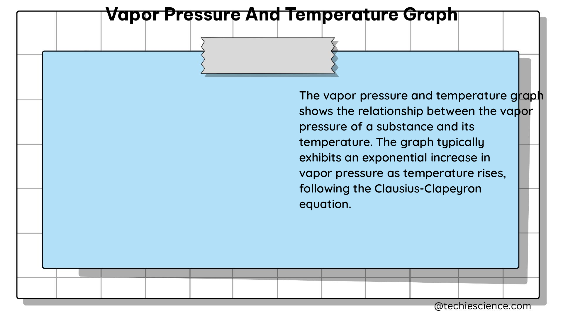
The graph shows the exponential relationship between the vapor pressure and temperature of water. As the temperature increases, the vapor pressure increases exponentially, as predicted by the Clausius-Clapeyron equation.

Technical Specifications for Vapor Pressure and Temperature Graphs

To create a high-quality vapor pressure and temperature graph, you should follow these technical specifications:

  1. Software Tools: The graph can be created using various software tools, such as Excel, MATLAB, or Python.
  2. Scales: The graph should have a logarithmic scale for the vapor pressure and a linear scale for the temperature.
  3. Axis Labels: The x-axis should be labeled “Temperature (°C)”, and the y-axis should be labeled “Vapor Pressure (kPa)”.
  4. Graph Title: The graph should include a title, such as “Vapor Pressure Curve of Water”.
  5. Data Points: The data points should be accurately plotted on the graph.
  6. Curve Fitting: The curve should be fitted using a suitable method, such as the Antoine equation or the Clausius-Clapeyron equation. The curve should be smooth and continuous, and it should pass through the data points as closely as possible.

By following these technical specifications, you can create a high-quality vapor pressure and temperature graph that effectively communicates the relationship between these two important properties.

Additional Data and Considerations

In addition to the water example, vapor pressure and temperature graphs can be created for a wide range of substances, including other common liquids and gases. The specific data points and curve shapes will vary depending on the substance’s properties, such as the molar enthalpy of vaporization and the critical temperature.

It’s also important to note that the Clausius-Clapeyron equation is valid only for the liquid-vapor equilibrium region, and it may not accurately describe the vapor pressure behavior near the critical point or in the supercritical region.

Conclusion

The vapor pressure and temperature graph is a fundamental tool in understanding the behavior of substances in different conditions. By understanding the theoretical relationship between vapor pressure and temperature, as well as the technical specifications for creating these graphs, you can effectively analyze and interpret the behavior of various substances. This comprehensive guide has provided you with the necessary knowledge and resources to become an expert in vapor pressure and temperature graphs.

References

  1. Chemistry LibreTexts. (2020, October 27). 7.2: Vapor Pressure – Chemistry LibreTexts. Retrieved from https://chem.libretexts.org/Courses/Oregon_Institute_of_Technology/OIT:_CHE_202_-_General_Chemistry_II/Unit_7:_Intermolecular_and_Intramolecular_Forces_in_Action/7.2:_Vapor_Pressure
  2. Penski, E.P., & Latour, Jr., L.J. (1971). Conversational Computation Method for Fitting the Antoine Equation to Vapor-Pressure-Temperature Data; EATR 4491; U.S. Army Chemical Research Laboratory: Edgewood Arsenal, Aberdeen Proving Ground, MD, 1971; UNCLASSIFIED Report (AD881829).
  3. Seber, G.A.F., & Wild, C.J. (2003). Nonlinear Regression. John Wiley & Sons.
  4. NIST/TRC Web Thermo Tables. (n.d.). Retrieved from https://webbook.nist.gov/chemistry/
  5. Lide, D.R. (Ed.). (2005). CRC Handbook of Chemistry and Physics (86th ed.). CRC Press.

The Ultimate Guide to Choosing the Perfect Camera Lens for Landscape Photography

camera lens for landscape photography

In the world of landscape photography, the choice of camera lens is a critical decision that can make or break the final image. The lens you select not only determines the field of view and perspective but also plays a crucial role in capturing the desired composition, story, and relationship between the elements in the … Read more

The Ultimate Guide to Choosing the Perfect Lens for Wildlife Photography

lens for wildlife photography

When it comes to capturing the beauty and majesty of the natural world, wildlife photography is a genre that requires specialized equipment and techniques. At the heart of any successful wildlife photography setup is the lens, which plays a crucial role in bringing distant subjects within reach and allowing for close-up shots of elusive creatures. … Read more

The Ultimate Guide to Choosing the Perfect Lens for Street Photography

lens for street photography

Street photography is a captivating genre that requires a unique approach to capturing the essence of everyday life. The choice of lens plays a crucial role in shaping the visual narrative and the overall aesthetic of your street photographs. In this comprehensive guide, we will delve into the technical details and practical considerations that will … Read more

Astrophotography with Telescopes: A Comprehensive Guide for Physics Students

astrophotography with telescopes

Astrophotography with telescopes is a captivating field that combines the art of photography with the science of astronomy. By harnessing the power of telescopes and advanced imaging techniques, astrophotographers can capture breathtaking images of celestial objects, from distant galaxies to stunning nebulae. This comprehensive guide will delve into the technical aspects of astrophotography, providing physics … Read more

Slope Of Position Time Graph: Exhaustive Insights And FACTS

Screenshot 2021 11 24 100241 300x261 1

The graph is the representation of any two physical quantities with respect to each other. This article is about the slope of position time graph

A position-time graph of an object represents position and time on the two respective axes. It infers how far an object moves in a given time. The slope of position and time graph represents the velocity of the subject. From the points on the slope, we can find the velocity at a given time. 

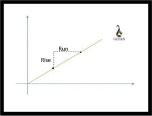
The steepness of the slope tells about the direction of the given quantity. Just by looking at the slope, you can know a lot about the given graph. To calculate the slope of the graph, take two points on the line. Draw the vertical line from one point that is known as rising, and a horizontal line from another called to rise. The slope thus is the ratio between the rise and run, that is:

slope=rise/run

pic 1 new
Slope of the graph
pic 2 3
Positive and Negative Slope

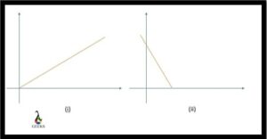
From moving from left to right, if the slope runs upward, as shown in figure (i), then it is taken as positive. If the slope runs downward, as shown in figure (ii), then it is taken to be negative. 

What is the slope of position time graph

For the position and time graph, we take one quantity on the x-axis and the other one on the y-axis. It determines the motion of the object, i.e. from the graph, we get to know about its position at any particular time. The steepness, length and shape of the graph determine how an object is moving. 

The slope of position time graph is found by plotting the graph, and then on joining the points, we get a line either rising up or down. This line is the slope of the graph. By following the steps described above, we can determine the value of the slope. 

What does the slope position-time graph signify

The slope of the position-time graph reveals the magnitude of the velocity of a moving particle. It tells vital information about the velocity of a particular object. For instance, a small slope signifies a smaller velocity; a negative one leads to a negative value of velocity. 

At the same time, a constant slope determines the constant velocity, and if the slope keeps changing, that is, a curved line leads to a changing velocity. Therefore the slope of a position-time graph can be positive, negative, constant or changing by making a curved line. The value can also be zero in case the slope line is parallel to the time axis. 

Screenshot 2021 11 24 100241
Slope of position time graph

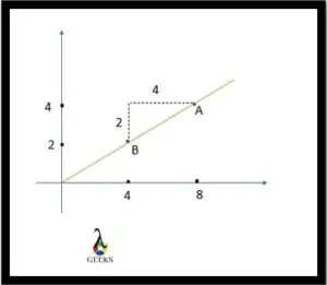
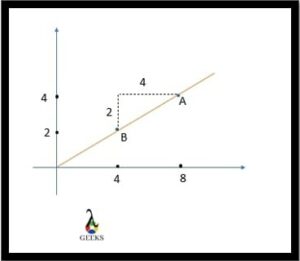
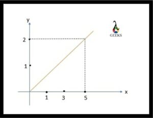
Suppose we are given the position-time graph as above, now; to determine the slope of the graph, we take two points as A and B on the line. From these two points, we draw perpendicular lines. The next step is to calculate the slope as:

slope=rise/run

CodeCogsEqn 19

Therefore the velocity of the object in that particular time would be 2 m/s. 

Screenshot 2021 11 24 100335

For the above graph, how will we find the position of the body when time equals 5 seconds. We can see that when the time t = 5 seconds, the position axis is marked at 2 m. Therefore the position of the object is 2 meters in 5 seconds. 

What is slope of a position vs time graph called

The slope of the position vs time graph is called velocity; it is also termed as displacement per unit time. The slope of this graph is determined as:

dx/dt=Displacement/time

We know the displacement/ time gives us the value of velocity. Therefore we have;

dx/dt=velocity

Hence its unit equals m/s. If the slope is steeper, it tells that the velocity is greater. 

If the position of the graph is increasing with time, then the slope is also positive velocity. Then the velocity increases or remains constant. If the velocity increases, then the body is accelerating.

 If the position is decreasing with time, the slope gives negative velocity. Which eventually means that body is decelerating. 

Slope of position time graph
Positive and Negative Slope of Position Time Graph

In the above figure, the first figure (i) shows the positive velocity and upward slope. At the same time, the second slope (ii) with a downward slope determines the negative velocity. 

Screenshot 2021 11 24 100737
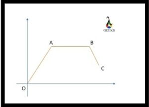
Variations in the slope

In the above figure from O to A, the slope is positive, then from A to B it is zero and at last from B to C, the slope is negative. 

What is the use of position-time graph

The slope of position time graph is used to find the velocity of the given object. It is simpler to find the average velocity using the graph. The graph depicts the motion of any given body.

By plotting the graph, we can find the position at the given time and time at the given position. Graphical representation is an effective way of finding detailed information about the motion of a body in a small and efficient way. 

Screenshot 2021 11 24 100539
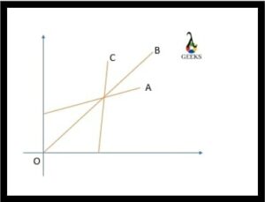
Motion of 3 Persons

In the above graph, the position-time of 3 persons A, B and C are plotted. It is clearly visible that the slope of B is the greatest; hence its velocity is the highest. Secondly, we can see that the line of all the three persons intersects at point P, which means that they will be at that same position in the given time. 

Therefore, the slope of position time graph is very useful to know all about the motion of two or more objects with respect to each other. It tells about the distance of the object at a particular time.  

What does the intercept of a position-time graph represent

The points where the graph intersects the x-axis and y-axis are known as intercepts.

The position-time graph has two axes and thus two intercepts. One is an x-intercept, and the other one is a y-intercept. Where the line of slope strikes the x-axis (horizontal) is called an x-intercept, whereas the y-intercept is defined as the point where the graph intersects the y-axis (vertical).

If we take the position on the y-axis, then the y-intercept tells about the starting position of the moving object. At that instant, time would be zero. 

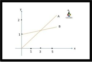
Screenshot 2021 11 24 100453

To understand this, take a look at the graph above. Two cars start at the same time. Car A has its initial position as 0, but car B has its initial position of 1 cm as its line has a y-intercept at 1. 

Similarly, if we take the time on the x-axis, then the point where the graph will intersect will be the x-intercept of time. At this point, the position of the moving object would be zero. 

How does a position vs time graph look

In the position time graph, the x-axis denotes the time, and on the y-axis, the position is depicted. Look at the above figure; it is the position time graph. This is how the graph looks. Let’s try to plot a graph and understand it better. 

Screenshot 2021 11 24 100414
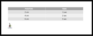
Table showing the motion of a car

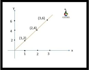
The above table shows us the data of a moving car. The position of the car at different intervals of time is given. Now, let us take the time on the x-axis and position it on the y-axis. Now start plotting the points. 

Screenshot 2021 11 24 100649

Once you have plotted all the given coordinates, the last thing is to join them, and you will get the required position-time graph. 

Slope of position time graph of the object is at rest

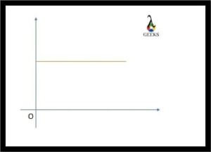
We have talked about the slope being rising up, down and curved. Now for an object at rest, what would be the value of the slope, and how will it look?. Well, for the rest object, the slope is zero. 

Screenshot 2021 11 24 100615
The slope is parallel to x-axis

When the slope of the position-time graph is zero, it means that the body is not moving at all. Therefore we get the graph as the line parallel to the time axis that is the x-axis. It means that the object’s position will remain the same for the different time periods. 

Frequently Asked Question (FAQs)

What is a position-time graph? 

A graph is a mathematical and visual representation of any two or three physical quantities. 

Position-time time graph is the representation of the position and time of a moving object. It describes the motion of the body. The graphical representation is useful by telling us about the position of the moving body in a given time.  

What physical quantity do we calculate by the slope of the position time graph? 

By calculating the slope of the position and time graph, we get the value of velocity.

The slope of any moving body is calculated as:

Slope = change in vertical value/ change in horizontal value

Which gives the value of the velocityThe unit of velocity is m/s. 

Can the slope of the position-time graph be negative?

Yes, the slope of the position and time graph can be negative. 

It depicts the negative velocity of the body. When moving from left to right, if the slope moves downward, then the value of it would be negative, which is possible. The slope can be negative, positive, zero, or keep ls changing. 

Is slope always straight for the position-time graph?

The slope of the position and time graph does not always have to be straight. 

The straight slope depicts that either the velocity is increasing or decreasing. The slope can be curved; this tells that the velocity is continuously changing. The line of slope can be either be straight or curved. 

What information does the position-time graph provide?

With the position-time graph, you can know all about the motion of a particle.

By finding the slope of the position and time graph, we get to know all about the motion of the body. The negative slope indicates negative velocity. It also tells about the starting position of the object. 

How will we know that the object is not moving from the position-time graph? 

The slope can either be negative, positive or zero. 

The slope would be zero when the line of graphs is parallel to the time axis. This would mean that the position of the object remains the same for different times; that is, it is not moving.  

Also Read: